Aside: Why the ACF and PACF Look the Way They Do in an MA(1) Process
Introduction
By now you know the AR and MA models and roughly what each one is doing to a series. This aside slows down on one particular case, the MA(1), and asks why its ACF and PACF end up looking the way they do on the page.
An MA(1), the same one-lag moving-average model from the ARMA chapter, is:
\[
y_t = \theta \epsilon_{t-1} + \epsilon_t
\]
\(\epsilon_t\) is the white-noise shock at time \(t\), the word we have been using since the autocorrelation chapter, and \(\theta\) is the MA coefficient. The equation never mentions \(y_{t-1}\), and yet \(y_t\) and \(y_{t-1}\) still end up correlated. That correlation comes entirely from the shock the two values share, \(\epsilon_{t-1}\), not from any direct dependence of one on the other. Shared noise versus direct dependence is the whole story of this aside.
Two things about the PACF of an MA(1) trip people up. The lag-1 PACF undershoots the true \(\theta\), and the lag-2 PACF is usually negative even though the model has no lag-2 term anywhere in it. Both are real, both are explainable, and simulation is the fastest way to see them before we derive them.
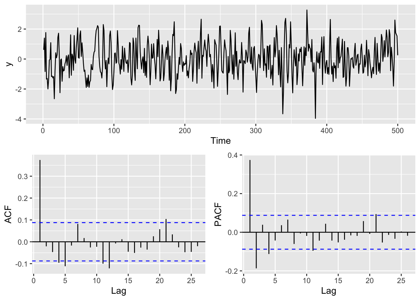
The series itself is choppy at short range and nothing more, the signature of a process with one lag of memory and no more. The ACF drops sharply after lag 1, the MA(1) fingerprint from the ARMA chapter. The PACF is the interesting one: a modest bump at lag 1, then a dip below zero at lag 2 that has no business being there if you read the model equation literally. That dip is what the rest of this aside explains.
That is the MA(1) pattern in a nutshell: the ACF spikes at lag 1 and drops off fast, and the PACF spikes smaller at lag 1 and then dips negative at lag 2.
Simulation Study Across Many MA(1) Coefficients
One simulation is a single data point. To see the pattern instead of a coincidence, draw \(\theta\) at random from \([0.2, 0.9]\) a thousand times, simulate an MA(1) for each draw, and keep the PACF at lags 1 and 2.
Code
m <-1000# Number of simulationsres <-matrix(NA, m, 3) # Object to store theta, PACF lag 1, PACF lag 2thetas <-runif(m, 0.2, 0.9) # Randomly draw MA(1) coefficients for simulationres[, 1] <- thetas # Store thetafor (i in1:m) { y <-arima.sim(model =list(ma = thetas[i]), n = n) # Simulate MA(1) tmp <-Pacf(y, plot =FALSE) # Get PACF res[i, 2] <- tmp$acf[1, 1, 1] # Store lag 1 PACF res[i, 3] <- tmp$acf[2, 1, 1] # Store lag 2 PACF}res <-as.data.frame(res)names(res) <-c("simulatedTheta", "pacfLag1", "pacfLag2")
The Lag-1 PACF Undershoots \(\theta\)
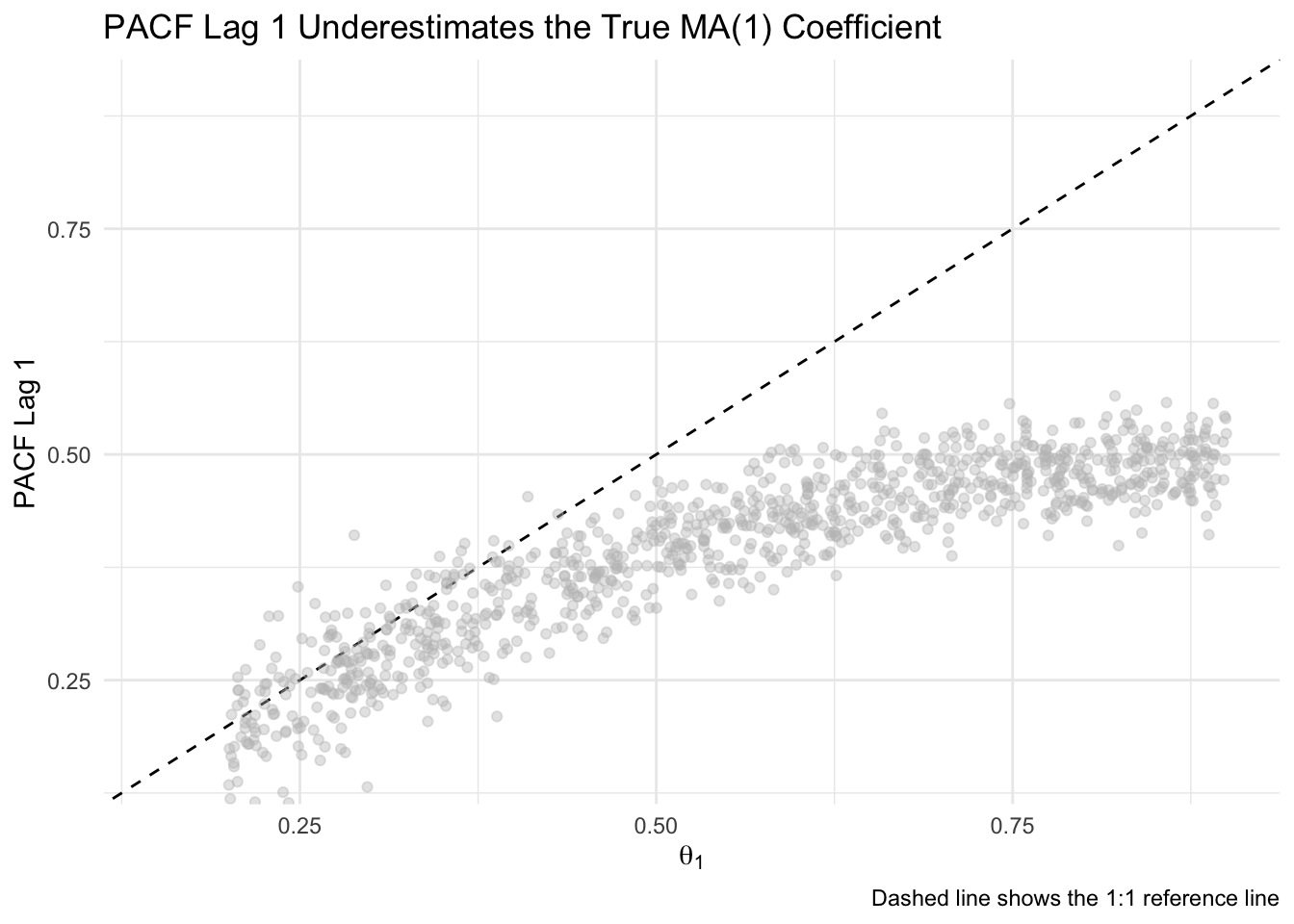
Plot the true \(\theta\) against the PACF value each simulation produced at lag 1. If the PACF were just reading off \(\theta\), every point would sit on the dashed 1:1 line. It doesn’t. The PACF grows more slowly than \(\theta\) does, and the gap widens as \(\theta\) climbs.
Code
ggplot(res, aes(x = simulatedTheta, y = pacfLag1)) +geom_abline(slope =1, intercept =0, linetype ="dashed") +geom_point(alpha =0.4, color ="gray") +labs(x =expression(theta[1]),y ="PACF Lag 1",title ="PACF Lag 1 Underestimates the True MA(1) Coefficient",caption ="Dashed line shows the 1:1 reference line" ) +coord_cartesian(xlim =c(0.15, 0.9), ylim =c(0.15, 0.9)) +theme_minimal()
Why This Happens
The PACF at lag 1 is just the coefficient from regressing \(y_t\) on \(y_{t-1}\), which for lag 1 is also the plain ACF. In an MA(1), \(y_t\) and \(y_{t-1}\) correlate because they share \(\epsilon_{t-1}\), not because one causes the other. That is a weaker kind of relationship than the direct dependence an AR(1) has, so it makes sense that it undershoots \(\theta\).
Work out that correlation directly and you get
\[
\rho(1) = \frac{\theta}{1 + \theta^2}
\]
which is always smaller than \(\theta\) itself (try \(\theta = 1\): \(\rho(1) = 0.5\)) and grows more slowly as \(\theta\) climbs. That formula falls out of the covariance and variance directly. The covariance between \(y_t\) and \(y_{t-1}\) is \(\theta \sigma^2\), the one shock they share. The variance of \(y_t\) is \(\sigma^2(1 + \theta^2)\), because \(y_t\) is built from two independent shocks, \(\epsilon_t\) and \(\theta \epsilon_{t-1}\), whose variances add. Divide the two, the \(\sigma^2\) cancels, and you are left with \(\theta / (1 + \theta^2)\).
Call this underestimation if you like, but it isn’t bias in the statistical sense. The PACF at lag 1 is doing exactly what it is supposed to: measuring correlation, not handing back a model parameter.
The simulation bears this out. PACF lag 1 rises as \(\theta\) does, but it never reaches the 1:1 line, exactly as the formula predicts.
The Lag-2 PACF Goes Negative
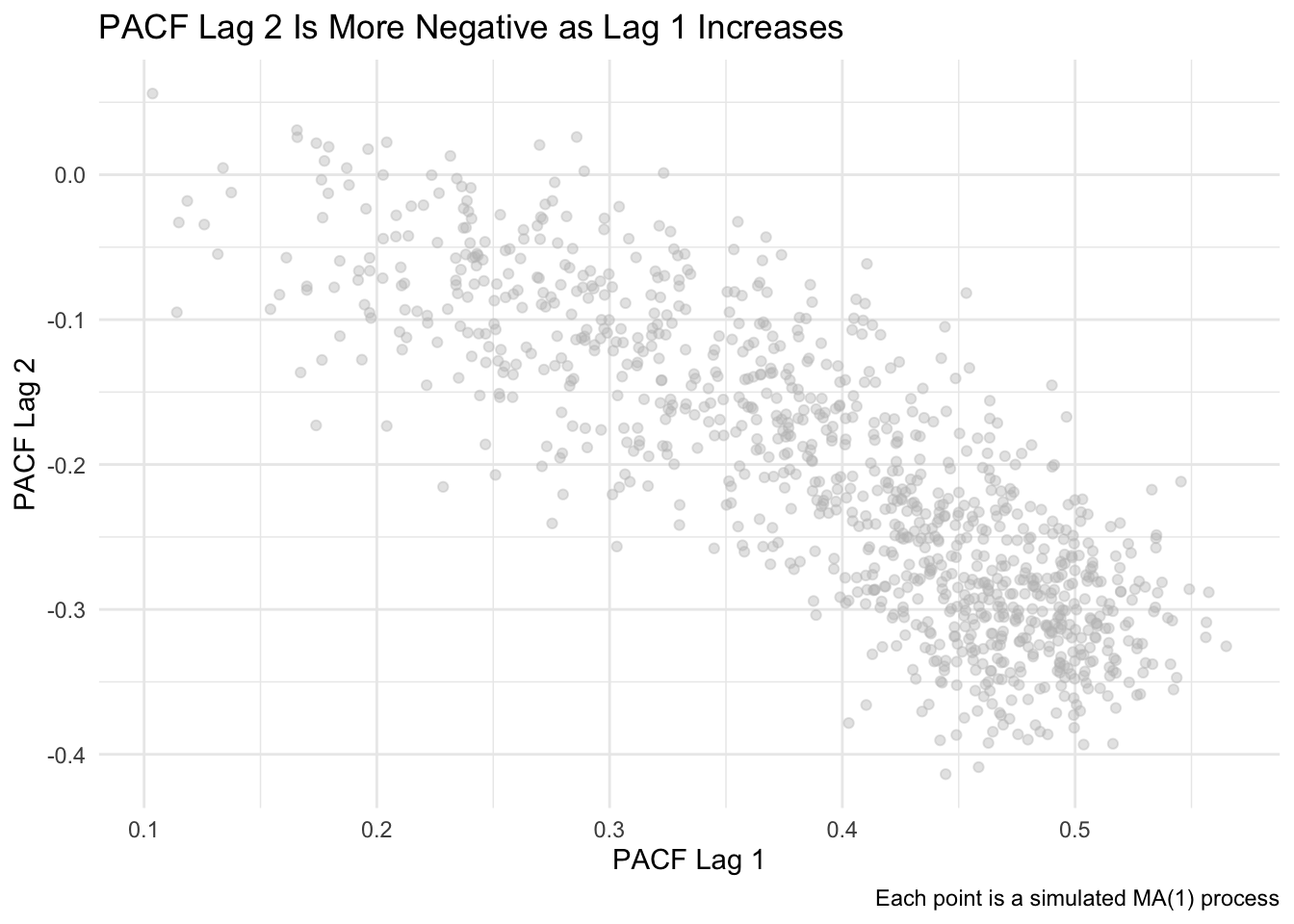
Plot PACF lag 2 against PACF lag 1 across the same thousand simulations and a clean inverse relationship falls out: the bigger lag 1 gets, the more negative lag 2 gets. That is the model’s one-lag memory showing up a second time, this time as a correction.
Code
ggplot(res, aes(x = pacfLag1, y = pacfLag2)) +geom_point(alpha =0.4, color ="gray") +labs(x ="PACF Lag 1",y ="PACF Lag 2",title ="PACF Lag 2 Is More Negative as Lag 1 Increases",caption ="Each point is a simulated MA(1) process" ) +theme_minimal()
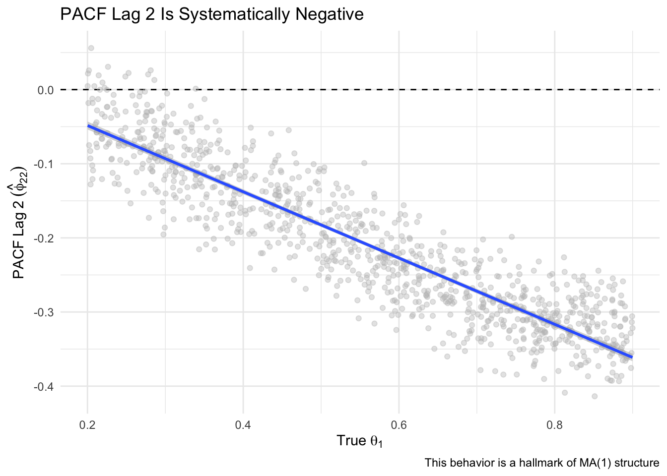
Plot it against the true \(\theta\) instead and the slope is just as clean: more \(\theta\) means a more negative lag-2 partial, a systematic pattern and not simulation noise.
Code
# Also show vs thetaggplot(res, aes(x = simulatedTheta, y = pacfLag2)) +geom_hline(yintercept =0, linetype ="dashed") +geom_point(alpha =0.4, color ="gray") +geom_smooth(method ="lm") +labs(x =expression(True ~ theta[1]),y =expression(PACF ~ Lag ~2~ (hat(phi)[22])),title ="PACF Lag 2 Is Systematically Negative",caption ="This behavior is a hallmark of MA(1) structure" ) +theme_minimal()
Why This Happens
The PACF at lag 2 is the partial correlation between \(y_t\) and \(y_{t-2}\) once \(y_{t-1}\) has been accounted for. The MA(1) equation has no \(y_{t-2}\) term at all, so where does that correlation come from? Through the middleman. \(y_{t-2}\) carries \(\epsilon_{t-2}\), which shows up again in \(y_{t-1}\), and \(y_{t-1}\) is exactly the thing being held constant.
Once you condition on \(y_{t-1}\), whatever is left of \(y_{t-2}\)’s relationship to \(y_t\) runs the other way, and the coefficient comes out negative. That negative pull gets stronger as \(\theta\) grows, which is the near-linear downward slope in the plot above.
There is a closed form for this. Solve the Yule-Walker equations for a process with \(\rho(1) = \theta / (1 + \theta^2)\) and \(\rho(2) = 0\) (true for any MA(1), since the model has no memory past lag 1), and the lag-2 partial autocorrelation comes out to
A word on notation before you go further. \(\phi_{kk}\) is standard shorthand for “the PACF at lag \(k\),” and it is not the same \(\phi\) we have been using since the autocorrelation chapter for an AR coefficient. The two collide on purpose: for an AR(\(p\)) process, the PACF at lag \(p\)is the last AR coefficient, \(\phi_{pp} = \phi_p\), so Box and Jenkins reused the symbol deliberately rather than by accident. Here, in an MA(1) with no AR part at all, \(\phi_{22}\) is pure PACF and nothing more. The Durbin-Levinson recursion (see the aside on PACF by hand) is what actually computes it: the unique contribution of \(y_{t-k}\) to predicting \(y_t\) once you have controlled for every intermediate lag, \(y_{t-1}\) through \(y_{t-(k-1)}\).
Plug in a few values of \(\theta\) and you get the same negative, steepening curve the simulation drew.
Where This Shows Up
Two things to carry forward. The lag-1 PACF undershoots \(\theta\) because it is picking up shared noise, not a direct dependency. The lag-2 PACF goes negative because the shock at \(t-2\) has to route through \(y_{t-1}\) to reach \(y_t\), and that routing flips sign once \(y_{t-1}\) is held fixed. Both are why the ARMA chapter could tell you, without deriving it there, that an MA process’s PACF decays and oscillates instead of cutting off cleanly the way an AR process’s does. Now you know why, and you know better than to read a PACF value as a stand-in for a model parameter.