Aside: A Glimpse of Cross-Spectral Analysis

Introduction

The cross-correlation chapter asked which of two series leads the other, and answered in time: producers a step ahead of grazers. The spectral analysis chapter was asking a different question about a single series: not when (time domain), but how often (frequency domain). Put the two questions together and there’s a natural one left over: does the lead between two series depend on which cycle you’re looking at? A slow multi-year wobble and a sharp seasonal spike could easily lead and lag by different amounts, and a single cross-correlation lag can’t tell them apart. That’s cross-spectral analysis. It deserves a fuller treatment than there’s room for here, but it’s worth knowing it exists.

library(tidyverse)
library(PNWColors)

bookPal <- pnw_palette("Sunset2", n = 5, type = "discrete")

From One Series to Two

spectrum(), the function this chapter has leaned on the whole way through, is itself a thin wrapper around a lower-level function, spec.pgram(). Feed spec.pgram() a single series and it does exactly what spectrum() has been doing all along. Feed it two columns bound together instead, and it estimates two new things at every frequency: coherence and phase.

Coherence is an ordinary correlation, just computed one cycle length at a time instead of once for the whole record. A plain correlation coefficient asks whether two series move together across everything they do; coherence asks the narrower question of whether the part of each series that repeats every twelve months moves together, ignoring whatever the three-month part or the two-year part are doing. It even keeps a similar scale, 0 to 1, like a squared correlation, where 0 means the two series have nothing to do with each other at that cycle length and 1 means they move in lockstep at it.

Phase only means something once coherence says there’s a relationship worth describing. Picture two gears turning at the same rate, that’s what high coherence at a frequency amounts to, both series completing one cycle in the same span of time. Phase asks whether the teeth line up: does a peak in one series land on a peak in the other, or does one lag a quarter turn behind? It’s reported as an angle, a fraction of one full turn, rather than directly in months, because the same angle stands for a different stretch of time depending on which frequency you’re looking at.

Try it on a pair with a stronger, more famous story to tell than a soft food-web lead: the lynx and the snowshoe hare from the ARMA chapter’s exercise, predator and prey, in pelts traded with the Hudson’s Bay Company from 1845 to 1935.

LynxHare <- readRDS("data/LynxHare.rds")

tibble(year = as.numeric(time(LynxHare)),
  Hare = as.numeric(LynxHare[, "Hare"]),
  Lynx = as.numeric(LynxHare[, "Lynx"])) |>
  pivot_longer(c(Hare, Lynx)) |>
  ggplot(aes(year, value, color = name)) +
  geom_line() +
  scale_color_manual(values = c(Hare = bookPal[1], Lynx = bookPal[5])) +
  labs(x = "Year", y = "Pelts traded (thousands)", color = NULL) +
  theme_minimal()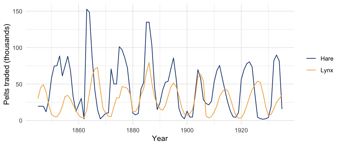

The two populations rise and fall together, boom and bust, with the lynx usually a beat behind the hare, exactly the coupling the classic predator-prey story predicts. Cross-spectral analysis can put a number on that beat.

xspec <- spec.pgram(cbind(LynxHare[, "Hare"], LynxHare[, "Lynx"]), spans = c(3, 3), taper = 0.1, plot = FALSE)

# the hare's own dominant cycle, from a plain univariate spectrum, independent of the cross-spectrum below
hareSpec <- spectrum(LynxHare[, "Hare"], span = 3, plot = FALSE)
cycleFreq <- hareSpec$freq[which.max(hareSpec$spec)]
cycleIdx <- which.min(abs(xspec$freq - cycleFreq))

tibble(freq = xspec$freq, coherence = xspec$coh) |>
  ggplot(aes(freq, coherence)) +
  geom_line(color = bookPal[1]) +
  geom_vline(xintercept = cycleFreq, linetype = "dashed", color = "grey40") +
  labs(x = "Frequency (cycle / year)", y = "Coherence",
    title = "Hare and lynx, coherence by frequency") +
  theme_minimal()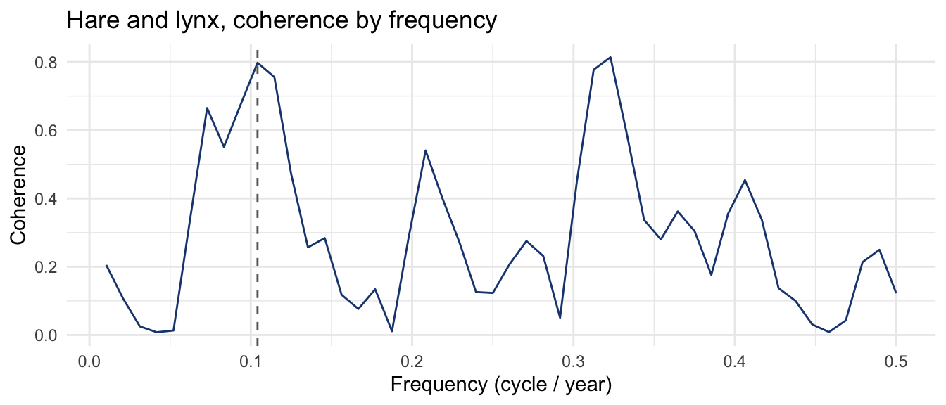

The dashed line marks the hare’s own dominant cycle, a period of about 9.6 years, found from nothing more than the hare’s own univariate spectrum, the same tool the spectral analysis chapter built. Coherence between hare and lynx at that exact frequency is 0.8, close to its ceiling of 1: whatever the hare’s ten-year boom and bust is doing, the lynx is doing it too. (There’s a taller peak further left in the plot, near a three-year period, but nothing in the ecology singles that one out the way the decadal cycle does, so it’s not the peak to focus on.)

Now look at whether the two gears are actually in step, and where.

tibble(freq = xspec$freq, phase = xspec$phase) |>
  ggplot(aes(freq, phase)) +
  geom_line(color = bookPal[5]) +
  geom_hline(yintercept = 0, color = "grey70") +
  geom_vline(xintercept = cycleFreq, linetype = "dashed", color = "grey40") +
  labs(x = "Frequency (cycle / year)", y = "Phase (radians)",
    title = "Hare and lynx, phase by frequency") +
  theme_minimal()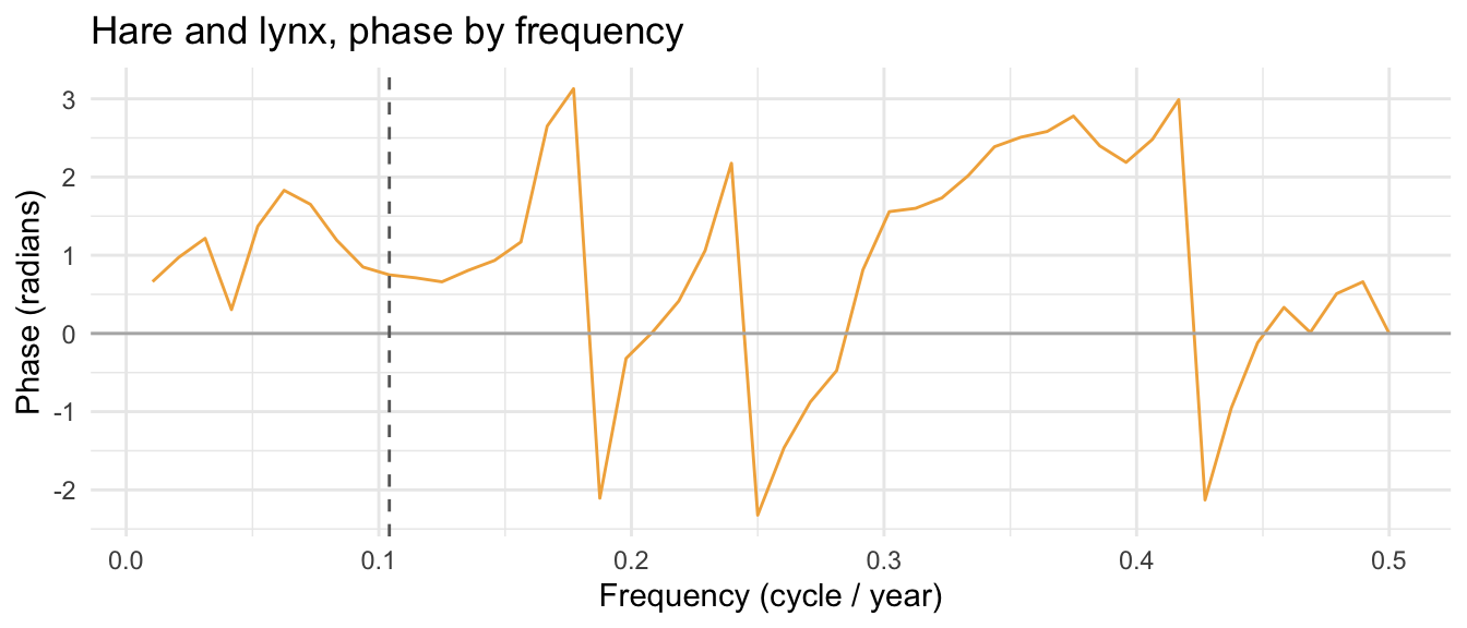

Away from the coherence peak this line is close to meaningless, bouncing between \(-\pi\) and \(\pi\) with no pattern, because phase only describes a relationship that exists in the first place; where coherence is near zero, “which one leads” is not a question with an answer. Read the two plots together, not the phase plot alone. At the one frequency where coherence actually earned its keep, the decadal cycle, the phase is 0.75 radians, about 0.12 of a full turn. Converting that fraction to time at this specific frequency puts it at 1.1 years, hare leading lynx. That’s the textbook predator-prey lag, recovered without ever sliding one series past the other in time: instead of reading a single best-matching offset off a cross-correlation plot, this reads a lead off the one cycle length where the two series are actually shown to be moving together.

That phase number would move if the smoothing span above changed, which is the catch with coherence: a raw, unsmoothed estimate is close to worthless (every frequency comes out with coherence 1, whether the series are related or not), so you’re always trading resolution for stability, the same trade this chapter made with span all along. Getting that trade right, and building a proper confidence interval around a coherence estimate before trusting a number this precise, is enough material for a book of its own; Shumway and Stoffer (2017) gives it the full chapter this aside couldn’t.