Forecasting

Big Idea

A forecast has two halves. The first half is the prediction: if a series leans on its own past, you can push that dependence forward and see where it is likely to go next. We built that skeleton back in the ARMA chapter. An AR or ARMA model is already a statement about how tomorrow relates to today, so turning it into a forecast is mostly bookkeeping. The second half is the part many people skip, and it is the only part that decides whether the first half was worth anything: checking the forecast against values it did not get to see. Hold back the end of a series, predict it from the rest, and compare. You never trust a forecast you have not backtested, because R will hand you a forecast whether or not it means anything. This chapter does both halves: it makes the prediction, and then sees if we believe it.

Packages

We stay with tsibble (Wang et al. 2020), tidyverse (Wickham 2023) for wrangling, and PNWColors (Lawlor 2020) for the figure colors. forecast (Hyndman et al. 2026) gives us the AR fitting and prediction tools and a tidy autoplot, and we read example data from CSV as usual.

library(tidyverse)
library(tsibble)
library(forecast)
library(PNWColors)

bookPal <- pnw_palette("Sunset2", n = 5, type = "discrete")

Forecasting an AR(1) by Hand

Start with the simplest process that has any memory at all, the AR(1):

\[ y_t = \phi y_{t-1} + \epsilon_t \]

with \(\phi = 0.7\) and \(\epsilon_t \sim \mathcal{N}(0, 1)\). The model says today is \(\phi\) times yesterday plus a fresh shock. If we know \(y_t\) and want \(y_{t+1}\), the shock has not happened yet and its expected value is zero, so the best one-step forecast is the deterministic part:

\[ \hat{y}_{t+1} = \phi y_t \]

That forecast is unbiased, but it is not certain. The error is whatever the shock turns out to be:

\[ e_{t+1} = y_{t+1} - \hat{y}_{t+1} = (\phi y_t + \epsilon_{t+1}) - \phi y_t = \epsilon_{t+1} \]

so the one-step error has the variance of a single shock, \(\text{Var}(e_{t+1}) = \sigma^2 = 1\). One step out, the uncertainty is just the noise.

Now push to two steps. We do not know \(y_{t+1}\), so we forecast it and feed our own forecast back in:

\[ \hat{y}_{t+2} = \phi \hat{y}_{t+1} = \phi^2 y_t \]

This is chained forecasting: each step uses the previous forecast as if it were data. It is what you have to do when the future is unknown, and it is where the uncertainty starts to compound. Expanding the true value,

\[ y_{t+2} = \phi(\phi y_t + \epsilon_{t+1}) + \epsilon_{t+2} = \phi^2 y_t + \phi \epsilon_{t+1} + \epsilon_{t+2} \]

the error now carries two shocks instead of one:

\[ e_{t+2} = \phi \epsilon_{t+1} + \epsilon_{t+2}, \qquad \text{Var}(e_{t+2}) = \phi^2 \sigma^2 + \sigma^2 = (0.49 + 1)\,\sigma^2 = 1.49 \]

Three steps out brings in a third shock, scaled by another power of \(\phi\), and the variance climbs to \(\phi^4 + \phi^2 + 1\). The pattern is a geometric series. For a \(k\)-step forecast from an AR(1) with white-noise variance \(\sigma^2\),

\[ \text{Var}(e_{t+k}) = \sigma^2 \sum_{j=0}^{k-1} \phi^{2j} \]

and because \(|\phi| < 1\), that series does not run off to infinity. It converges:

\[ \lim_{k \to \infty} \text{Var}(e_{t+k}) = \frac{\sigma^2}{1 - \phi^2} \]

The uncertainty grows with the horizon, but it levels off at a ceiling. For \(\phi = 0.7\) and \(\sigma^2 = 1\) the ceiling is \(1 / (1 - 0.49) \approx 1.96\), a standard deviation of about 1.4. This is the same geometric decay you saw in the AR(1) autocorrelation function, just read from the other end. The ACF told you how fast the past stops mattering; the forecast variance tells you how fast the future stops being knowable, and they are governed by the same \(\phi\).

So, as \(k\) grows, \(\hat{y}_{t+k} = \phi^k y_t\) decays toward zero, the mean of the process, while the interval fattens toward \(\sigma / \sqrt{1 - \phi^2}\), the standard deviation of the process. Far enough out, the model stops telling you anything useful and just hands you back the unconditional distribution of the series. I like to think about it as the forecast forgets where it started.

Let’s watch it happen. Simulate an AR(1), then chain the forecast forward from the last observed value and draw the interval as \(\pm\) one forecast standard deviation.

phi <- 0.7
sigma <- 1
n <- 60
h <- 25

set.seed(62)
epsilon <- rnorm(n)
y <- numeric(n)
y[1] <- epsilon[1]
for (t in 2:n) {
  y[t] <- phi * y[t - 1] + epsilon[t]
}

# chained forecast and its standard deviation, h steps out
fcSd <- function(k) sigma * sqrt(cumsum(phi^(2 * (0:(k - 1)))))
forecastDf <- tibble(
  time = (n + 1):(n + h),
  yhat = phi^(1:h) * y[n],
  sd   = fcSd(h)
)
observedDf <- tibble(time = 1:n, y = y)
ceilingSd <- sigma / sqrt(1 - phi^2)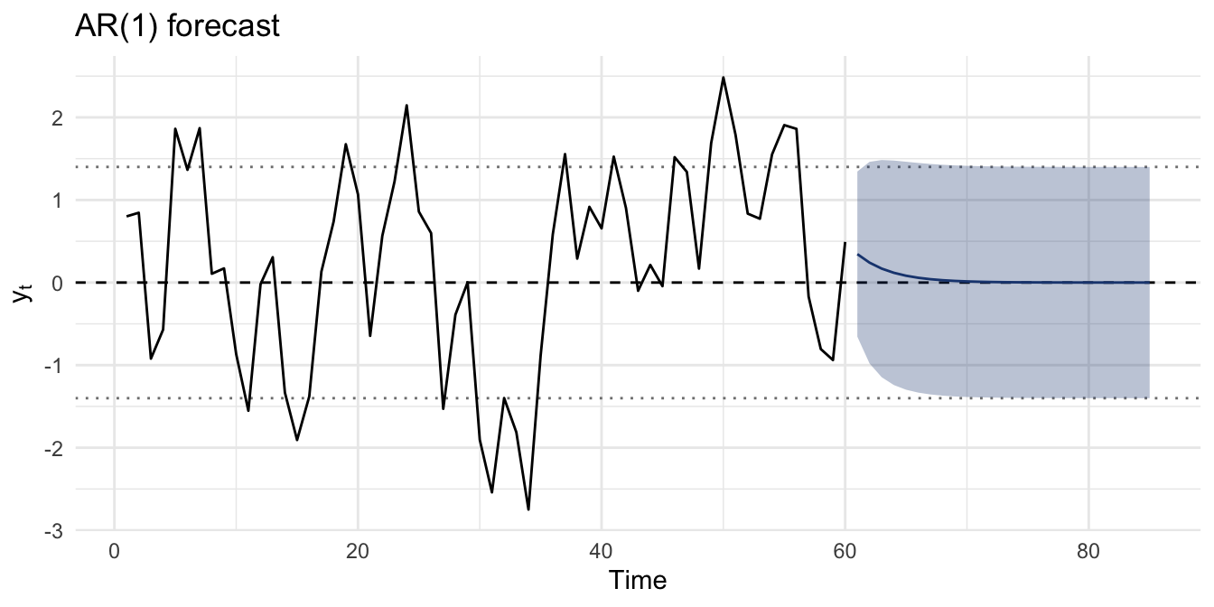

The navy forecast slides toward the mean and the band around it widens, fast at first and then hardly at all, flattening against the dotted lines that mark \(\pm\) the ceiling standard deviation. By ten or fifteen steps out the forecast has essentially given up and is reporting the long-run mean give or take the long-run spread. That is the shape of a forecast from a short-memory process: useful for a few steps, then asymptotically useless, and the math tells you exactly where the cutoff is.

The Forecast Runs Both Ways

Look again at the variance formula. There is no \(t\) in it and no sign that says which way time is running. \(\text{Var}(e_{t+k})\) depends on \(k\), the number of steps, not on the direction of the step. Nothing in the AR(1) machinery cares whether you are projecting into the future or into the past. An AR(1) is symmetric in time: the same \(\phi\) that links \(y_t\) to \(y_{t-1}\) links it to \(y_{t+1}\), so you can run the chain backward off the first observation exactly as you ran it forward off the last. Predict the prehistory of the series, and the forecast reverts to the same mean and the interval fattens to the same ceiling.

backwardDf <- tibble(
  time = (1 - h):0,
  yhat = rev(phi^(1:h) * y[1]),
  sd   = rev(fcSd(h))
)

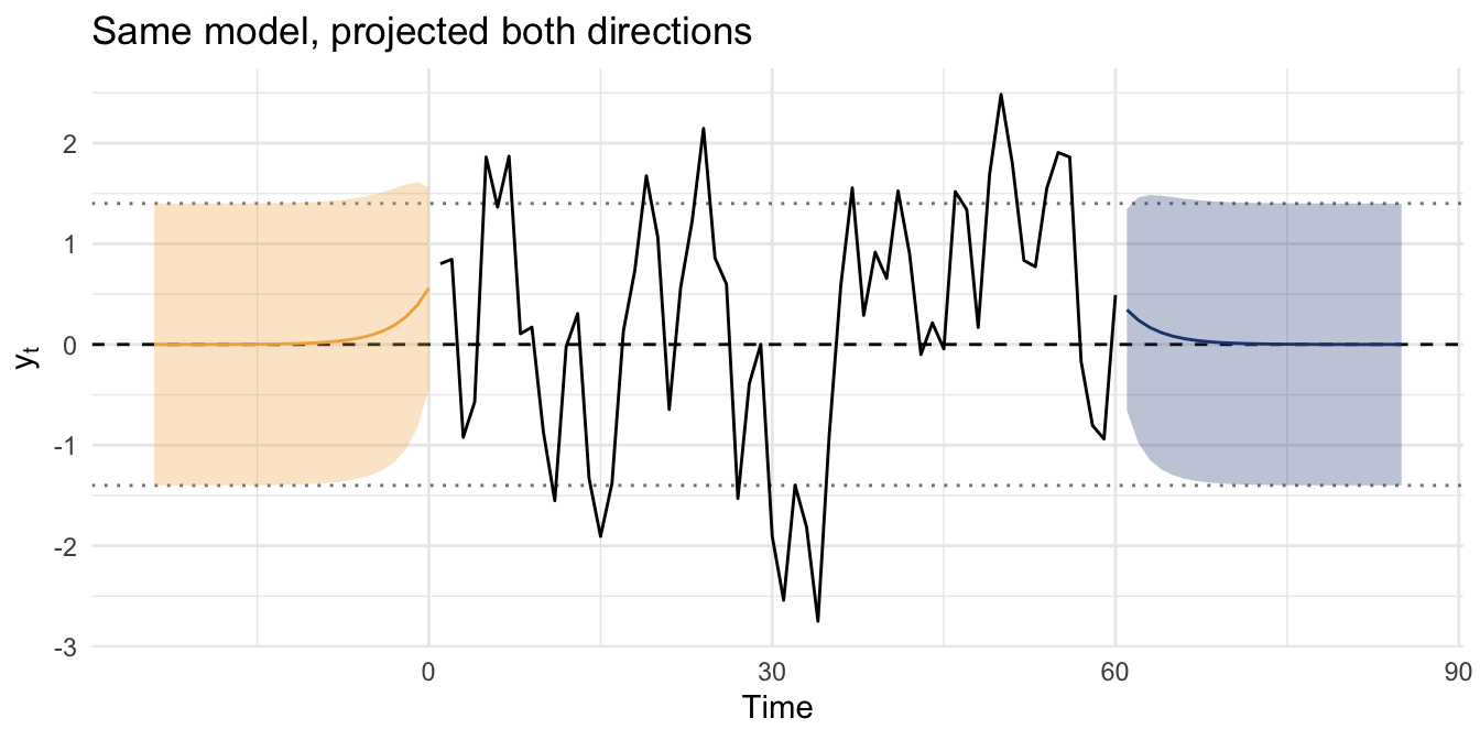
The gold forecast running off the left edge is a mirror of the navy one running off the right. Projecting backward to estimate values you never measured is hindcasting, or reconstruction, and it is how a paleoclimatologist turns a tree-ring width into a temperature for a year with no thermometer in it (next chapter!). The point to carry forward is that prediction does not have a preferred direction. The model is a statement about how neighbors in time relate, and you can lean on it to fill a gap on either side. The symmetry buys us something now: everything we are about to say about checking a forward forecast applies, unchanged, to checking a backward one.

A Forward Forecast: Sunspots

Synthetic data is obliging. Let’s forecast something measured. The annual sunspot count cycles over roughly eleven years, the kind of long, strong memory that gives a forecast something to grab. The record runs back to 1700.

data(sunspot.year)
autoplot(sunspot.year) +
  labs(x = "Year", y = "Sunspots (n)") +
  theme_minimal()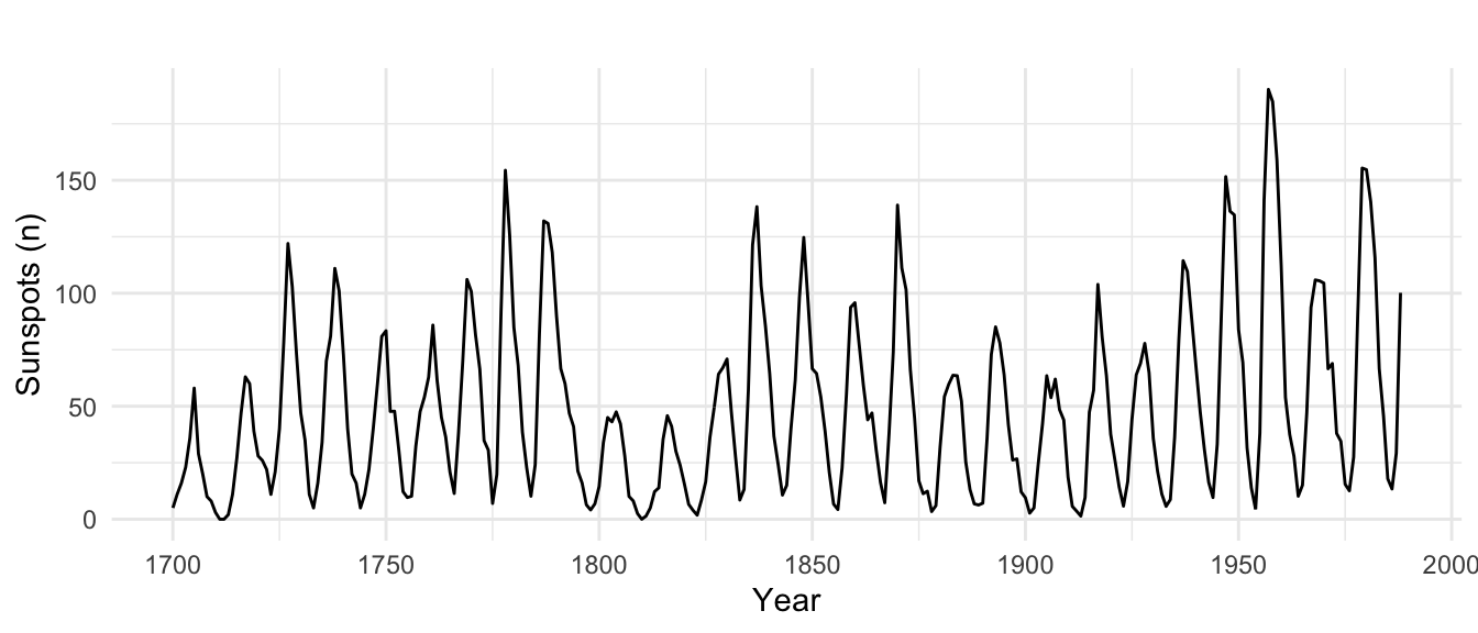

Up to now we have chosen model orders by hand, reading the ACF and PACF and comparing information criteria. That is the thoughtful way, because it makes you reason about the process. But you have probably found ar and auto.arima, which pick the order for you. We will use ar here. It fits a sequence of AR(p) models and keeps the one with the lowest AIC.

sunspotAr <- ar(sunspot.year)
sunspotAr$order

[1] 9

WarningThe blind algorithm

ar and auto.arima are convenient and dangerous. They optimize an information criterion until a stopping rule trips, and that is all they do. An information criterion rewards fit and penalizes parameters, but the penalty is not harsh enough when the sample is large or the noise is structured, so the algorithm will reach for a complicated model that fits the idiosyncrasies of your particular series rather than the process behind it. By default auto.arima will consider AR and MA orders up to five, plenty of room to fit noise. In a short series that can be reckless. And because near-identical scores can come from very different models, two runs on two samples of the same process can hand you two different stories. The criterion measures fit, not predictive skill, and those are not the same thing. Use these functions, but read what they return with suspicion, and never let one pick a model you cannot defend on mechanism. R prints an order either way.

Here ar landed on an AR(9), and for once the order is defensible. The sunspot cycle is solar physics, not an artifact, and nine years of memory on an eleven-year cycle is a model you can argue for. Most models have a predict method, so we forecast forward forty years and ask for the standard errors too.

sunspotFc <- predict(sunspotAr, n.ahead = 40)

forecastTb <- tibble(
  year  = as.numeric(time(sunspotFc$pred)),
  yhat  = as.numeric(sunspotFc$pred),
  lower = yhat - sunspotFc$se,
  upper = yhat + sunspotFc$se
)
observedTb <- tibble(
  year = as.numeric(time(sunspot.year)),
  y    = as.numeric(sunspot.year)
)

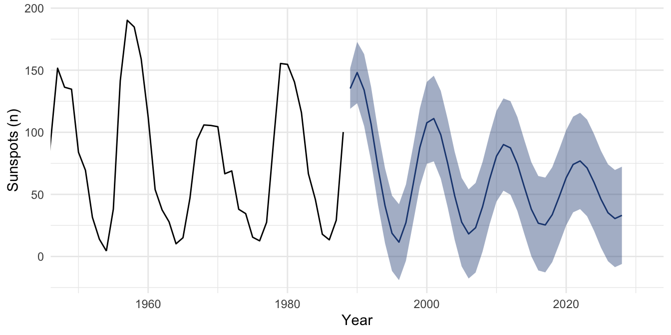
The AR(9) keeps the cycle going for a couple of oscillations, the peaks shrinking and the troughs filling as the forecast loses confidence, and the error band swelling around it. This is the AR(1) story from before, now with a longer memory: the forecast decays toward the mean and the interval fattens toward the ceiling, only the decay is slower and the path more interesting because the cycle takes a while to wash out. A few cycles ahead, the model has forgotten the phase and is reporting the average sunspot number with a wide band.

Now look harder at that band, because it is telling on itself. The error ribbon dips below zero in a dozen of those forty years, bottoming out around -19. A sunspot count cannot be negative. You cannot have fewer than no spots on the sun. The model does not know that. It was handed a column of numbers and a recipe for propagating Gaussian uncertainty, and nowhere in that recipe is the fact that the thing being counted has a floor at zero. The central forecast stays positive, but the interval wanders into territory that does not exist. This is the first conviction of the book in miniature: R will print a number whether or not it makes physical sense, and it falls to you to catch it. The fix is not exotic. You would forecast on a scale that cannot go negative, modeling the square root or the log of the count and transforming back, so the interval respects the floor. The lesson underneath it is bigger than sunspots. A forecast is only as sensible as the constraints you build into it, and a generic AR model builds in none. It does not know it is counting sunspots, or counting fish, or pricing a stock. It knows the numbers.

The plot looks impressive (for a short time anyway). Whether it is any good is a separate question, and the only way to answer it is to check.

Backtesting

So far we have admired forecasts without ever testing one. Every forecast in this chapter has run off the end of the data into territory where nothing can contradict it. That is the comfortable place to stop, and it is exactly where you fool yourself. The fix is to hold some data back. Split the series into a training piece and a testing piece, fit the model on the training piece only, forecast across the span you withheld, and compare the forecast to the values you were hiding. This is backtesting, and it is the same train-and-test discipline you would use on any model. The difference is that with a time series you cannot shuffle and split at random, because the order is the information. You withhold the tail.

Let’s do it somewhere the stakes are not hypothetical. Every year the International Pacific Halibut Commission has to set a catch limit before it knows how many young fish actually survived to join the population, so it forecasts recruitment: the number of fish, in thousands, entering the fishery that year. Forecast too high and the quota erodes a stock that cannot support it; forecast too low and you leave a sustainable harvest in the water. Fisheries agencies do exactly the kind of backtesting we are about to do, every season, because the alternative is finding out you were wrong after the boats have already gone out. It does not always work. When Newfoundland’s northern cod stock collapsed in 1992, the assessments feeding the catch quotas had been reading the population as healthier than it was for years, and that fishery has never recovered. A good backtest will not save you from every possible failure. It is still better than not checking at all.

halibut <- read_csv("data/halibut.csv", show_col_types = FALSE) |>
  filter(year >= 1935, year <= 1981)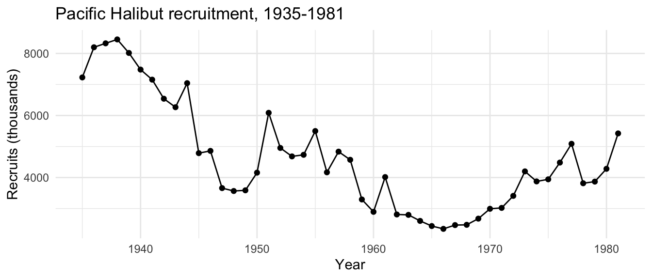

This is the recruitment record for Pacific Halibut, the big flatfish fished from Oregon to the Bering Sea and managed jointly by the US and Canada. It is annual, not monthly, so there is no season here for an algorithm to reconstruct out of stacked lags, only whatever year-to-year persistence cohort survival leaves behind. We hand the recruits column over as a ts and withhold the last ten years.

rec <- ts(halibut$rec, start = 1935, frequency = 1)

h <- 10  # withhold the last decade
recTrain <- head(rec, length(rec) - h)
recTest  <- tail(rec, h)

Fit an AR model on the training span and forecast across the test span.

recAr <- ar(recTrain)
recAr$order

[1] 1

arFc <- predict(recAr, n.ahead = h)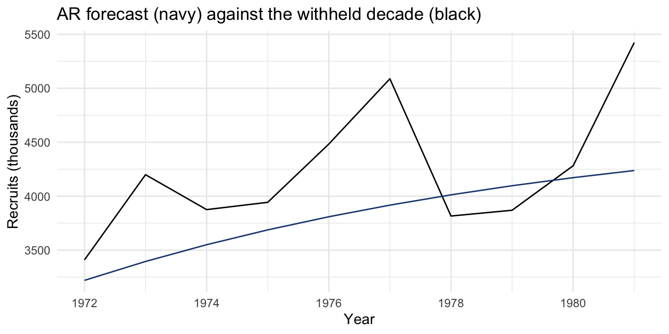

ar picked an order of one: a single year of memory. That is a model you can defend. Whatever drove one year class to survive tends to carry a little into the next, ocean conditions do not reset every January, and there is no twelve-month cycle sitting there for the algorithm to fake with a stack of lags. Put a number on the forecast.

arRMSE <- sqrt(mean((arFc$pred - recTest)^2))
arCor  <- cor(arFc$pred, recTest)
c(order = recAr$order, rmse = arRMSE, cor = arCor)

      order        rmse         cor 
  1.0000000 646.8914497   0.5587863 

Now ask what a very naive model could score. There is no season to hand a baseline for free here, so the fair baseline is simpler still: predict every withheld year with the training period’s long-run average recruitment, full stop.

meanPred <- rep(mean(recTrain), h)
meanRMSE <- sqrt(mean((meanPred - recTest)^2))
c(arRMSE = arRMSE, meanRMSE = meanRMSE)

  arRMSE meanRMSE 
646.8914 774.8970 

The AR(1) beats the flat average by a wide margin this time, not a rounding error. A strongly seasonal series can fake this kind of result cheaply: stack enough lags and an AR model reconstructs the annual cycle for free, and most of its apparent skill turns out to be the season itself, something a baseline that already knows the season matches almost as well. An annual recruitment series has no season to hand out for free, so the improvement here is actual signal, persistence in how one year’s recruitment leans on the last. It is a smaller, humbler forecast than the sunspot cycle, and it is exactly the kind of number a stock assessment leans on, an unglamorous edge over the flat average that still changes what catch limit looks defensible.

Holt-Winters

The AR model got its one lag of memory by fitting a coefficient the same way it would for any process, with nothing telling it that a recruitment series has a level that drifts and no season to speak of. A model built to handle level and trend on purpose, with parameters that mean something, ought to do at least as well. Holt-Winters forecasts by exponential smoothing, applied separately to the level, the trend, and (when there is one) the season, and the whole thing rests on one simple idea about weighted averages. Let’s build up to it from scratch so we can see the logic.

Suppose you have a short series and you want to predict the next value.

x <- 1:7
y <- c(8, 5, 12, 11, 12, 9, 19)
p1 <- ggplot(mapping = aes(x, y)) +
  geom_point() + geom_line() + lims(x = c(1, 9)) +
  theme_minimal()
p1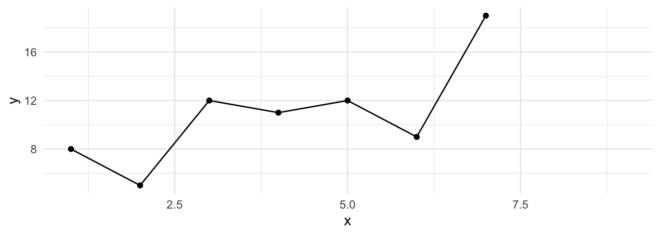

The plainest guess for \(\hat{y}_8\) is the mean of what you have. If \(y\) has a central tendency, predicting it to the average is not unreasonable. A small step up from there is a moving average that uses only the last few points instead of all of them, on the theory that recent values are more relevant. Either way, every point that goes into the average is weighted the same. The three-point moving average of \(y_5, y_6, y_7\) is

\[ \hat{y}_8 = \tfrac{1}{3} y_5 + \tfrac{1}{3} y_6 + \tfrac{1}{3} y_7 \]

which is the same sum-over-count you always compute, just written with the count moved up into each term. Written that way, it invites a question: why should the three weights be equal? In a time series we usually want recent points to count for more. So replace the equal weights with a vector of weights that sum to one, heavier near the present.

wma <- function(x, w) {
  nx <- length(x)
  nw <- length(w)
  sum(x[(nx - nw + 1):nx] * w)
}
wma(y, w = c(0.1, 0.2, 0.3, 0.4))

[1] 13.8

That predicts \(\hat{y}_8\) from the last four points with weights climbing toward the present:

\[ \hat{y}_8 = 0.1\,y_4 + 0.2\,y_5 + 0.3\,y_6 + 0.4\,y_7 \]

The weights have to sum to one or the answer drifts off scale. (This is exactly what stats::filter does with a weight vector, if you want to see the connection; we call it with the stats:: prefix because dplyr also has a filter.) Now take the idea to its limit. What if every point in the series contributed, with weights that shrink exponentially as you go back in time? Start with a smoothing coefficient \(\alpha = 0.9\) and let the weights be \(0.9, 0.9^2, 0.9^3, \dots\) going backward.

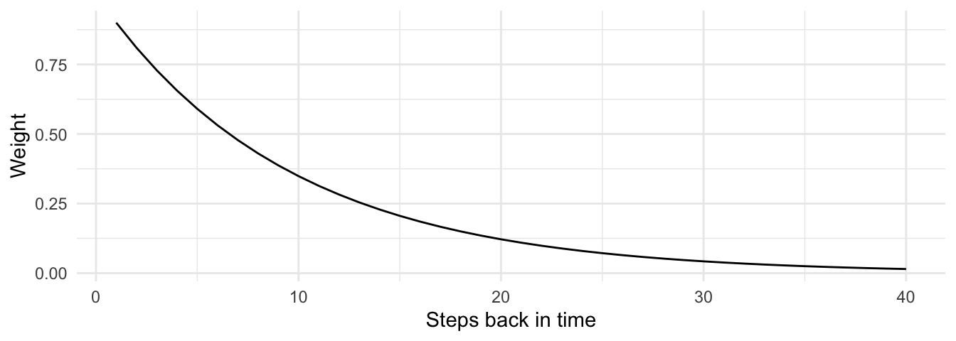
The weights decay smoothly to nothing, which is what we wanted, but there is a problem: they sum to more than one, so we cannot use them directly as a weighted average. Holt’s fix is clean. Write the smoothed value recursively:

\[ \hat{y}_t = \alpha\, y_t + (1 - \alpha)\, \hat{y}_{t-1} \]

Look at what that does. The new smoothed value is a weighted average of the current observation and the previous smoothed value, with weights \(\alpha\) and \(1 - \alpha\) that sum to one by construction. And because \(\hat{y}_{t-1}\) was itself built the same way from \(\hat{y}_{t-2}\), the recursion reaches all the way back, folding in every past value with a weight that decays geometrically. The infinite exponential weighting falls out of a two-term update. In a loop:

expSmooth <- function(x, alpha = 0.5) {
  xhat <- x[1]
  for (i in 2:length(x)) {
    xhat[i] <- alpha * x[i] + (1 - alpha) * xhat[i - 1]
  }
  xhat[length(x)]
}
expSmooth(y, alpha = 0.9)

[1] 18.02903

A large \(\alpha\) trusts the most recent point and barely smooths; a small \(\alpha\) leans on the accumulated history and smooths hard. That single dial is simple exponential smoothing. Holt-Winters runs three of these dials at once, one for the level (\(\alpha\)), one for the trend (\(\beta\)), and one for the season (\(\gamma\)), and adds them up into a forecast. The HoltWinters function finds the coefficients by numerical optimization, minimizing the squared one-step errors. We do not have to set them by hand.

Now put it on the halibut recruits, fit on the same training span, and backtest against the same withheld decade. There is no season in an annual series, so we turn the third dial off (gamma = FALSE) and let Holt-Winters run as plain level-plus-trend smoothing, Holt’s original method before Winters added the seasonal piece.

recHw <- HoltWinters(recTrain, gamma = FALSE)
hwFc <- predict(recHw, n.ahead = h)
hwRMSE <- sqrt(mean((hwFc - recTest)^2))
c(arRMSE = arRMSE, hwRMSE = hwRMSE, meanRMSE = meanRMSE)

  arRMSE   hwRMSE meanRMSE 
646.8914 628.9416 774.8970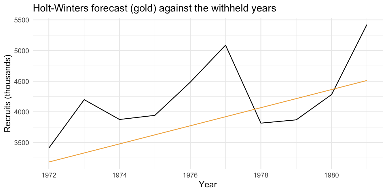 

Holt-Winters edges out the AR(1), and both clear the flat average by a wide margin. On held-out data the two dynamic models land close to one another, both leaning on the same year-to-year persistence, just weighting the recent past a little differently. If the numbers will not separate them, what does? Parsimony, mostly: two smoothing coefficients against one AR term is not much of a contest, and neither one reaches for more machinery than a single lag of memory can justify. The takeaway is smaller than the machinery: a stock’s recruitment carries some memory of the year before, not much, and a model that captures that little bit and nothing more is doing its job. Box’s line holds: all models are wrong, and the useful one here is the plain one you can explain to the people setting next year’s quota.

Do not mistake this for what a stock assessment actually looks like. What we just ran is two lines of R against forty-seven numbers. An actual halibut assessment folds in age structure, multiple fleets and gear types, tagging studies, survey indices with their own error, and increasingly a state-space model that separates the process noise in the population from the observation noise in how it was sampled, and it gets reviewed by a room of skeptical scientists before a quota comes out the other end. Fisheries forecasting is some of the hardest applied time series work in environmental science, and a fair amount of it is done by ecologists and statisticians who are better at this than the median econometrics PhD forecasting quarterly sales. An AR(1) and a two-parameter smoother will not get you hired at IPHC. They will get you far enough to recognize what the harder machinery is doing and why, which is a fine place for us to stop.

Wrapping Up

We forecast a series by pushing its own dependence forward, and we watched the uncertainty grow as a geometric series that saturates at a ceiling set by \(\phi\), the same coefficient that governs the ACF decay. We saw that the forecast has no preferred direction in time, which is the seed of reconstruction and the reason hindcasting is the same act as forecasting. And we made backtesting the centerpiece, because a forecast you have not checked against withheld data is a number R printed, not a result. Holding out the last decade of halibut recruitment and racing two models against a flat average showed a model beating the baseline because of persistence that was actually there, which is the kind of thing you only ever learn by checking, and the reason a fisheries agency runs this same discipline every season.

The split-sample idea, fit on part of the record and verify against the part you hid, is the engine of the reconstruction chapter next, which runs the same discipline backward instead of forward: calibrate on part of a long record, verify on the part held out, and only then trust the model to reach past the years anyone measured.

Exercises

Beat the climatology

Take the Bellingham weather record, data/kbli.csv, and build a monthly mean temperature series: read it as a tsibble, derive TAVG as the mean of TMAX and TMIN, and aggregate to monthly means with index_by and yearmonth. Convert it to a ts with frequency twelve and withhold the last three years. Fit an AR model and a Holt-Winters model on the training span, forecast across the withheld years, and compute the RMSE of each against the held-out data. Then build the climatology baseline, predicting each month by its training-period average, and compute its RMSE too. Does either model clear the baseline by enough to justify itself? Write a sentence on what that tells you about how much of the predictability in monthly temperature is just the season.

How far can you see?

The forecast-error variance of an AR(1) climbs to a ceiling of \(\sigma^2 / (1 - \phi^2)\). Simulate AR(1) series with \(\phi = 0.3\), \(0.7\), and \(0.95\), holding \(\sigma^2 = 1\). For each, compute the \(k\)-step forecast standard deviation out to fifty steps and find roughly how many steps it takes to reach 95 percent of the ceiling. How does that horizon change as \(\phi\) approaches one, and how does it line up with how slowly the ACF of each series decays? Use your answer to explain why a strongly autocorrelated series is both harder to forecast far out (a higher ceiling) and forecastable for longer (a slower approach to it).

Further Reading

• Cowpertwait and Metcalfe (2009), chapter 3, develops exponential smoothing and the full Holt-Winters method, including the trend and seasonal updates we only sketched, and works the algebra from the single smoothing equation up to the complete forecast.
• Hyndman and Athanasopoulos (2021) is the standard modern reference for forecasting in the tidy ecosystem. Its treatment of forecast evaluation, training and test splits, cross-validation, and accuracy measures is the natural next step past the single backtest we did here.