Stationarity

Big Idea

We ended the last chapter on a cliffhanger. An AR(1) process, \(y_t = \phi y_{t-1} + \epsilon_t\), has a coefficient \(\phi\) that we kept between -1 and 1, and every series we built came back to its mean sooner or later. The closer \(\phi\) sat to 1, the longer the memory and the slower the return. So push it to the wall. What happens when \(\phi = 1\)?

The series stops coming back to the mean. Each shock gets passed forward at full strength and never fades, the variance grows without bound, and the thing wanders off and never settles. That failure has a name, a unit root, and it breaks the one property most tools in the rest of this book assume: stationarity. This chapter is about what it means, the canonical way it fails, the difference between a trend you can subtract and a trend you have to difference away, and how to test whether your data have earned the assumption you are about to make of them.

Packages

We stay in the tsibble (Wang et al. 2020) framework from the earlier chapters, with tidyverse (Wickham 2023) and PNWColors (Lawlor 2020) as usual. forecast (Hyndman et al. 2026) gives us the ggplot-ready ACF we have been using, and tseries (Trapletti and Hornik 2026) carries the two unit-root tests at the end of the chapter.

Code

library(tidyverse)
library(tsibble)
library(forecast)
library(tseries)
library(PNWColors)

bookPal <- pnw_palette("Sunset2", n = 5, type = "discrete")

What Stationarity Means

A stationary series is one whose statistical character does not depend on when you look at it. Slide a window along the series, and the picture inside the window is the same wherever you put it: same average level, same amount of wiggle, same relationship between neighbors. Three constancies make that precise enough for our purposes.

The mean is constant. There is no trend. The series hovers around one level forever.
The variance is constant. The spread of the data this decade is the spread next decade. The wiggles do not grow or shrink over time.
The autocovariance depends only on the lag, not on absolute time. How strongly \(y_t\) relates to \(y_{t-k}\) is a function of the gap \(k\) alone. Lag-1 dependence is the same near the start of the record as it is near the end.

That is all we need. There is a stricter version that talks about the full joint distribution being invariant, and there is a measure-theoretic machinery underneath it, but the three items above are the working definition for everything we will do. When people say a series is stationary, this is usually what they mean.

Why fuss over it? Because the ACF and PACF you learned to read, the AR and MA coefficients you are about to fit, the standard errors a regression hands you, and the error bounds on a forecast are all derived under these constancies. A coefficient that describes how \(y_t\) leans on \(y_{t-1}\) only means something if that relationship is the same throughout the series. If the rules of the process drift as the series runs, a single set of fixed coefficients is describing an average of conditions that never actually held.

Here is what stationarity and three of its common failures look like.

Code

n <- 300
t <- 1:n

# stationary AR(1) phi 0.6
e <- rnorm(n)
stationarySeries <- numeric(n)
for (i in 2:n) stationarySeries[i] <- 0.6 * stationarySeries[i - 1] + e[i]

# a trend: the mean is not constant
trend <- 0.03 * t + rnorm(n)

# changing variance: the spread grows
hetero <- rnorm(n, sd = seq(0.2, 3, length.out = n))

# a random walk: wanders, never settles
walk <- cumsum(rnorm(n))

faces <- tibble(
  t = t,
  `Stationary AR(1)` = stationarySeries,
  `Trend (mean drifts)` = trend,
  `Changing variance` = hetero,
  `Random walk` = walk
) |>
  pivot_longer(-t, names_to = "series", values_to = "value") |>
  mutate(series = factor(series, levels = c("Stationary AR(1)",
    "Trend (mean drifts)",
    "Changing variance",
    "Random walk")))

faces |>
  ggplot(aes(t, value)) +
  geom_line(linewidth = 0.3) +
  facet_wrap(~series, scales = "free_y") +
  labs(x = "Time", y = NULL) +
  theme_minimal()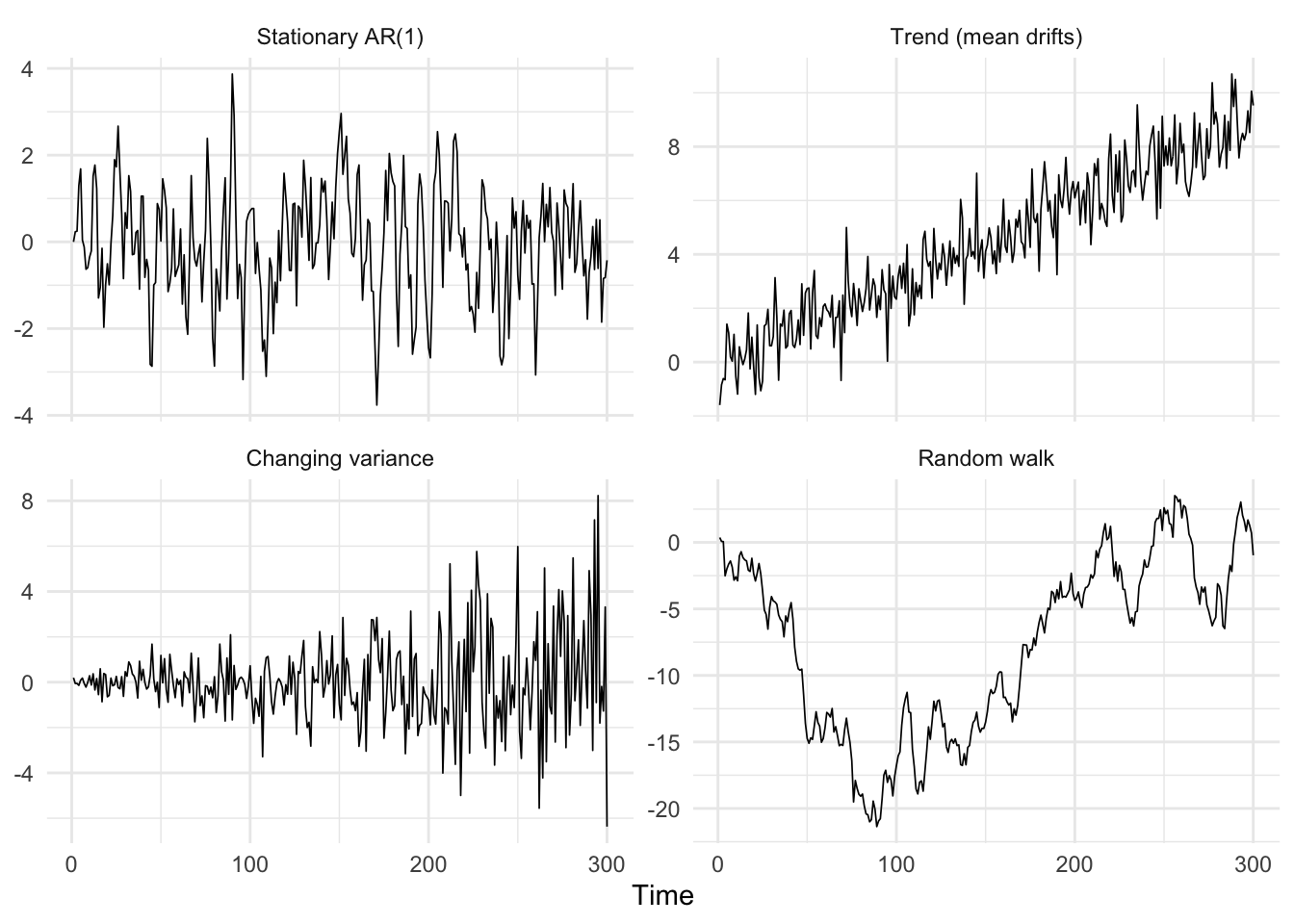

Only the top-left panel is stationary. The others each break one of the constancies, and the rest of the chapter is mostly about the bottom-right one, the random walk, because it is the sneakiest. A trend or a fan of growing variance announces itself. The random walk can look like an innocent meandering series with a trend that is not really there.

When \(\phi = 1\): the Random Walk

Let’s answer the cliffhanger directly. Take the AR(1) recursion and set \(\phi = 1\):

\[ y_t = y_{t-1} + \epsilon_t \]

Because the coefficient is 1 we can leave it out and read the equation plainly: each value is the previous value plus a fresh shock. Nothing pulls the series back toward a mean, because there is no \(\phi < 1\) doing the pulling. The series simply accumulates its shocks. This is the random walk, the canonical non-stationary process, and the unit root we flagged in passing at the start of the chapter. That odd name is worth a word.

Why is it called a unit root?

The name points at a single number: one. Forget the shocks for a moment and ask what an AR(1) does with one disturbance. A bump today is worth \(\phi\) a step later, \(\phi^2\) the step after, \(\phi^k\) after \(k\) steps. When \(|\phi| < 1\) those powers shrink toward zero, so the bump fades and the series forgets its past. That is the stationary case. When \(|\phi| > 1\) the powers blow up and the series explodes. The boundary between forgetting and exploding sits at exactly \(\phi = 1\), where \(\phi^k = 1\) for every \(k\): the bump never fades and never grows, it just stays, and the shocks pile up. That boundary value of one is the “unit” in unit root.

The “root” half is the more formal version of the same fact, the spot where a certain polynomial built from the model has a root of size one, and it takes a little linear algebra to set up. We do not need it here, but if you want to go further the idea lives under “the characteristic equation” and “the unit circle” in any time-series text.

A drift term \(\delta\) can be added to tilt the accumulation in one direction:

\[ y_t = \delta + y_{t-1} + \epsilon_t \]

Build one and you can watch it refuse to settle.

Code

n <- 300
walk <- numeric(n)
for (i in 2:n) walk[i] <- walk[i - 1] + rnorm(1)

ggplot(tibble(t = 1:n, walk), aes(t, walk)) +
  geom_line() +
  labs(x = "Time", y = expression(y[t]), title = "A random walk") +
  theme_minimal()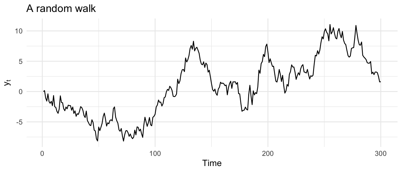

Run that a dozen times and you’ll see that you’ll get a dozen different shapes, some climbing, some sinking, some doubling back. That is the field mark. A stationary AR(1) always looks like the same animal no matter the seed. A random walk looks like anything.

There is a clean way to see why it is not stationary. Unwind the recursion from a start of zero and a random walk is just the running sum of all the shocks so far, \(y_t = \epsilon_1 + \epsilon_2 + \cdots + \epsilon_t\). The shocks are independent with variance \(\sigma^2\), so the variance of the sum is \(t\sigma^2\). The variance grows in direct proportion to how far you are into the series. The second constancy is broken by construction. We can confirm it by simulating many walks and looking at the spread across them at each time step.

Code

reps <- 2000
walks <- replicate(reps, cumsum(rnorm(n)))   # n x reps matrix

tibble(t = 1:n, empirical = apply(walks, 1, var)) |>
  ggplot(aes(t)) +
  geom_line(aes(y = empirical), color = bookPal[1]) +
  geom_abline(slope = 1, intercept = 0, linetype = "dashed") +
  labs(x = "Time", y = "Variance across realizations",
    title = "Random-walk variance grows with time") +
  theme_minimal()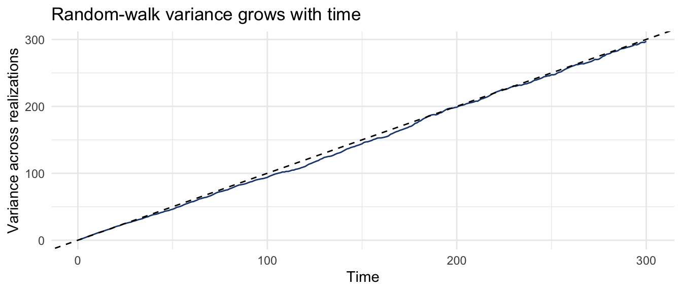

The empirical variance tracks the dashed line of slope one, exactly the \(t\sigma^2\) we derived with \(\sigma = 1\). A process whose variance you cannot pin down without also telling me what time it is cannot be stationary.

The autocorrelation of a random walk has a signature worth being able to spot. Back in the last chapter I asked you what the ACF and PACF of a random walk would look like. Here is the answer.

Code

ggAcf(walk) + labs(title = "ACF of a random walk") + theme_minimal()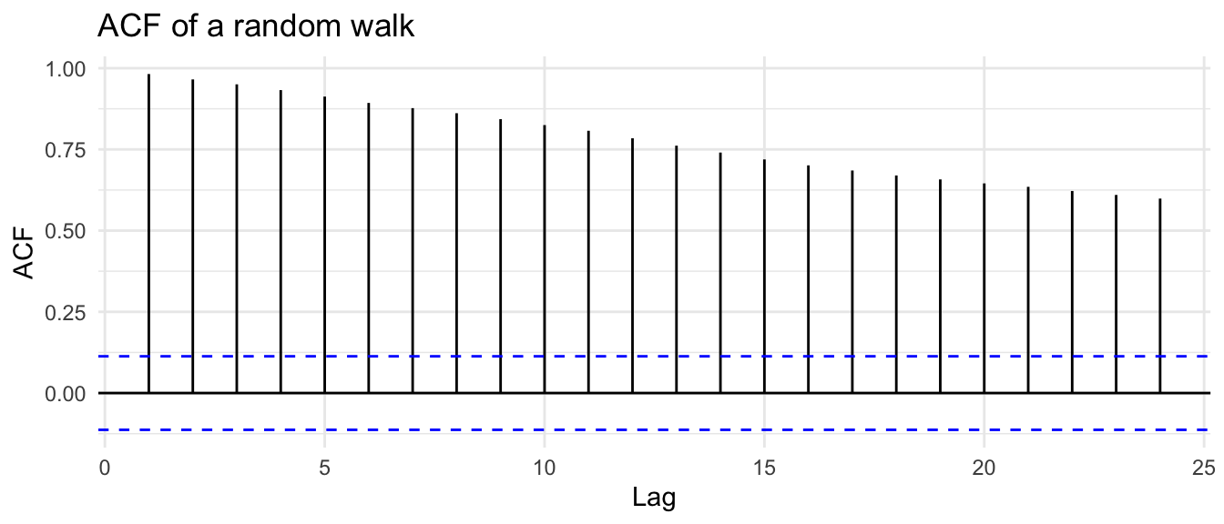

The ACF starts near one and comes down slowly, almost a straight ramp, staying significant for many lags. Compare that to the AR(1) from last chapter, where the ACF fell off geometrically and was back to nothing within a handful of lags. Slow, nearly linear ACF decay that refuses to die is the fingerprint of a series with a unit root. Once you have seen it a few times you will start to recognize it on sight, which is the point of building these by hand.

Two Kinds of Trend

Now the idea this whole chapter is built to deliver, and the one that decides whether you reach for an ARMA model or an ARIMA model. There are two completely different things people call a trend, they can look identical on a plot, and they need opposite repairs.

A deterministic trend is a fixed function of time with stationary noise riding on top. The series is tied to a line (or a curve); the level at time \(t\) is set by the clock, and the fluctuations around it are well-behaved. A series like this is called trend-stationary, because once you remove the trend, what is left is stationary.

A stochastic trend is the random walk we just described. There is no underlying line. The apparent trend is the accumulation of shocks, and a different set of shocks would have wandered somewhere else entirely. A series like this is called difference-stationary, because differencing it (taking \(y_t - y_{t-1}\)) is what makes it stationary.

Here are two series, one of each kind, built to rise at the same rate.

Code

n <- 200
t <- 1:n

# trend-stationary: a fixed line plus stationary AR(1) noise
e <- rnorm(n)
ar <- numeric(n)
for (i in 2:n) ar[i] <- 0.6 * ar[i - 1] + e[i]
detTrend <- 0.05 * t + ar

# difference-stationary: a random walk with the same drift
stochTrend <- numeric(n)
for (i in 2:n) stochTrend[i] <- 0.05 + stochTrend[i - 1] + rnorm(1)

tibble(t, `Deterministic trend` = detTrend,
  `Stochastic trend` = stochTrend) |>
  pivot_longer(-t, names_to = "series", values_to = "value") |>
  ggplot(aes(t, value)) +
  geom_line() +
  facet_wrap(~series) +
  labs(x = "Time", y = NULL) +
  theme_minimal()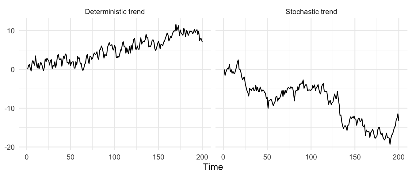

Look at those for a moment and try to say which is which without the labels. You cannot, reliably. Both climb, both wobble on the way up, both would tempt you to draw a straight line through them and call it a trend. But one of those lines is a feature of the process and the other is an accident of one particular sequence of random shocks.

The repairs are not interchangeable. For the deterministic trend, you subtract the trend. Fit a line against time and keep the residuals.

Code

detResid <- resid(lm(detTrend ~ t))
ggplot(tibble(t, detResid), aes(t, detResid)) +
  geom_line() +
  labs(x = "Time", y = "Residual", title = "Detrended deterministic series") +
  theme_minimal()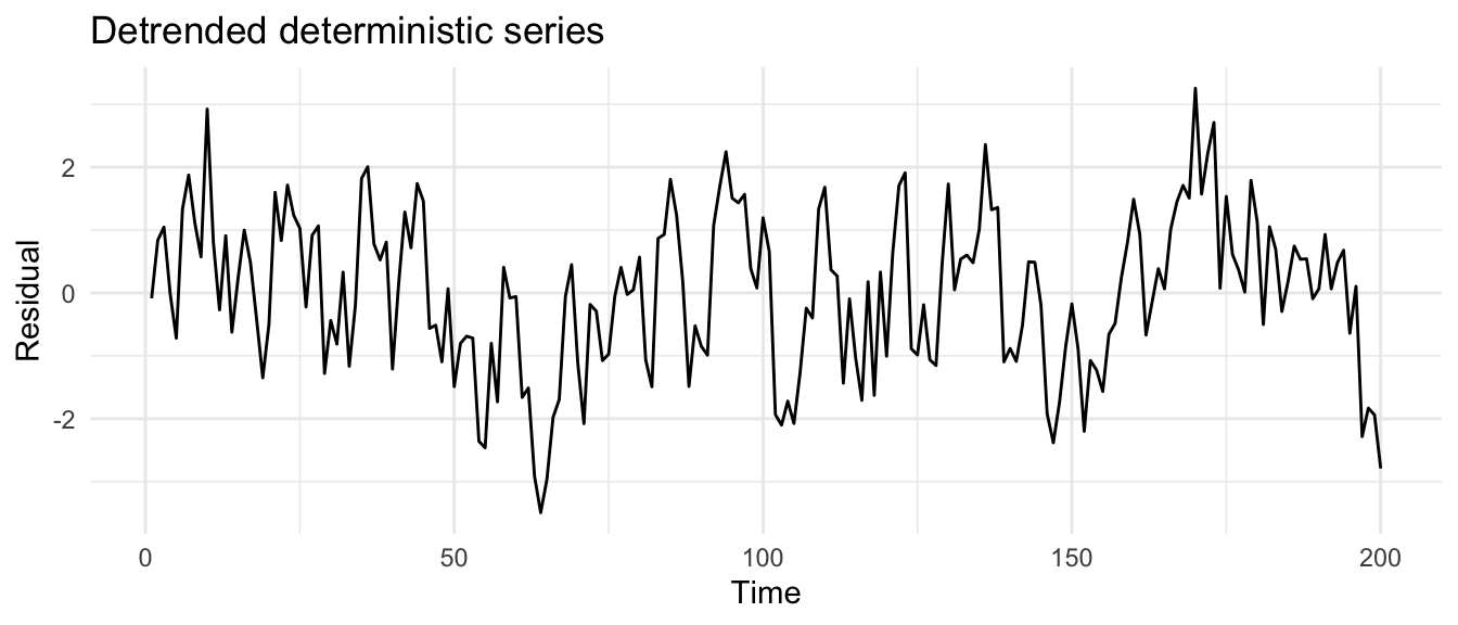

That residual series is flat, centered, and stationary. Detrending was the right move. Now watch what happens when you try the same trick on the stochastic-trend series.

Code

stochResid <- resid(lm(stochTrend ~ t))
ggplot(tibble(t, stochResid), aes(t, stochResid)) +
  geom_line() +
  labs(x = "Time", y = "Residual",
    title = "Random walk after subtracting a fitted line") +
  theme_minimal()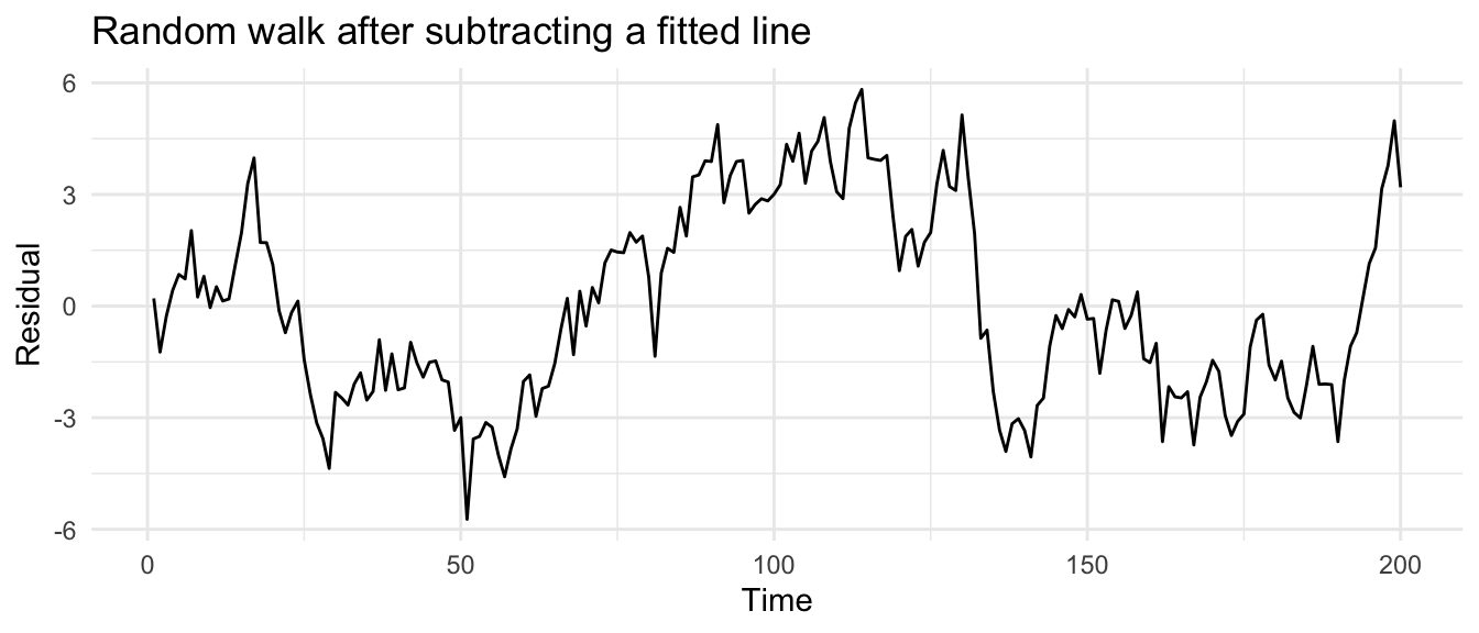

Subtracting the line did not fix it. The residuals still wander in long slow excursions, because there was no line there to remove in the first place. The lag-1 autocorrelation of those residuals is still about 0.92, almost as persistent as the original. Detrending a stochastic trend leaves you with a non-stationary series and a false sense that you handled it.

The right repair for the stochastic trend is differencing.

Code

stochDiff <- diff(stochTrend)
ggplot(tibble(t = 2:n, stochDiff), aes(t, stochDiff)) +
  geom_line() +
  labs(x = "Time", y = expression(y[t] - y[t - 1]),
    title = "Differenced stochastic series") +
  theme_minimal()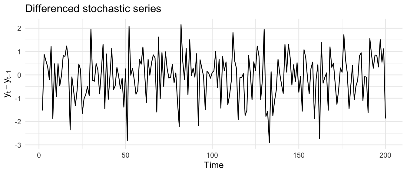

Differencing cancels the accumulation. Since \(y_t = \delta + y_{t-1} + \epsilon_t\), the difference \(y_t - y_{t-1}\) is just \(\delta + \epsilon_t\), white noise around the drift. The series is stationary and we can finally model it.

The two repairs do not commute, and using the wrong one has a cost in both directions. Detrend a stochastic trend and, as we just saw, you have not removed the problem. Difference a deterministic trend and you overdifference: you inject a spurious moving-average wobble into a series that was already fine once detrended. The lesson is not to pick a favorite repair and apply it everywhere. The lesson is to figure out which kind of trend you have. That is what the tests in the next section are for, and it is the whole reason ARIMA keeps differencing separate from the AR and MA parts. The “I” in ARIMA is this decision. More about that in the next chapter.

Testing for a Unit Root: ADF and KPSS

Your eye is a good instrument, and “plot your data” remains the first commandment. But the two trends in the last section looked the same, and eyeballing cannot always separate a slow stationary wander from a stochastic trend. There are two standard tests that help, and the most useful thing to understand about them is that they ask opposite questions.

The Augmented Dickey-Fuller test (ADF) takes non-stationarity as its null hypothesis. Its null is “there is a unit root.” A small p-value lets you reject that and conclude the series is stationary. So for ADF, small p is good news.

The KPSS test runs the other way. Its null is “the series is stationary.” A small p-value rejects stationarity and flags a unit root. So for KPSS, small p is the warning.

Reading them together is the right habit, because the two nulls cover each other’s blind spots. When ADF rejects and KPSS does not, both point to stationary, and you can relax. When ADF fails to reject and KPSS rejects, both point to a unit root, and you should difference. When they disagree, the series is telling you it is ambiguous, often a short record or something hovering near \(\phi = 1\), and no single p-value is going to resolve it for you.

Let’s plant a unit root and watch the tests earn their keep. We simulate a random walk, run both tests on it, then difference it and run both again. Here is the series we planted.

Code

planted <- cumsum(rnorm(300))   # a known unit root
ggplot(tibble(t = seq_along(planted), planted), aes(t, planted)) +
  geom_line() +
  labs(x = "Time", y = expression(y[t]), title = "A planted unit root") +
  theme_minimal()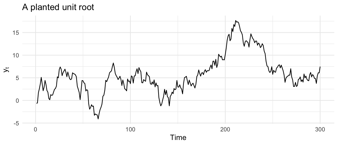

It wanders, which is what a random walk does. Now run both tests on it.

Code

adf.test(planted)               # null: unit root. want SMALL p to reject


    Augmented Dickey-Fuller Test

data:  planted
Dickey-Fuller = -2.2852, Lag order = 6, p-value = 0.4561
alternative hypothesis: stationary

Code

kpss.test(planted)              # null: stationary. SMALL p flags a unit root


    KPSS Test for Level Stationarity

data:  planted
KPSS Level = 1.7365, Truncation lag parameter = 5, p-value = 0.01

The ADF p-value is large, so it cannot reject a unit root. The KPSS p-value is at its floor, so it rejects stationarity. Both tests agree: this series has a unit root. We know they are right, because we built it that way. Now difference it. The differenced series should be the white-noise shocks the walk was accumulating, with no trend left to speak of.

Code

plantedDiff <- diff(planted)
ggplot(tibble(t = seq_along(plantedDiff), plantedDiff), aes(t, plantedDiff)) +
  geom_line() +
  labs(x = "Time", y = expression(y[t] - y[t - 1]),
    title = "The planted walk, differenced") +
  theme_minimal()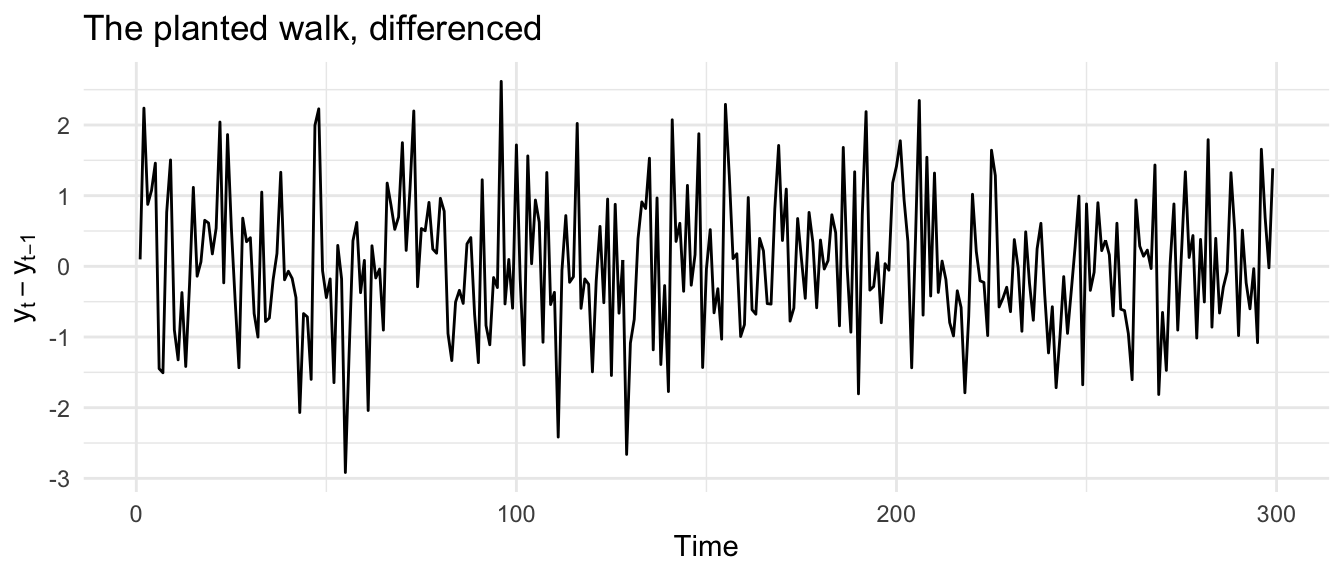

That looks like noise around a flat line, which is the point. Run the tests again.

Code

adf.test(plantedDiff)


    Augmented Dickey-Fuller Test

data:  plantedDiff
Dickey-Fuller = -6.5031, Lag order = 6, p-value = 0.01
alternative hypothesis: stationary

Code

kpss.test(plantedDiff)


    KPSS Test for Level Stationarity

data:  plantedDiff
KPSS Level = 0.062639, Truncation lag parameter = 5, p-value = 0.1

The verdicts flip. ADF now rejects the unit root, KPSS no longer rejects stationarity, and the differenced series passes both. We planted a unit root, the tests caught it, we differenced it out, and the tests cleared. That is the planted-signal loop in miniature, and it is exactly the workflow you run on data whose history you do not already know.

A note on the warnings these functions throw. When a p-value is past the edge of the table the test interpolates from, R tells you the true p-value is smaller (or larger) than the printed one. That is not an error. A KPSS p printed as 0.01 with a warning means “0.01 or less,” which only strengthens the conclusion.

An Observed Series: Lake Huron

Simulated data always cooperates. Let’s run the same workflow on something measured. Back in the first chapter, Lake Huron’s annual water level was our example of a ts object. We never asked whether it was stationary. Now we can.

Code

data(LakeHuron)
huron <- as_tsibble(LakeHuron)
huron |>
  ggplot(aes(index, value)) +
  geom_line() +
  labs(x = "Year", y = "Level (feet)",
    title = "Lake Huron annual water level, 1875-1972") +
  theme_minimal()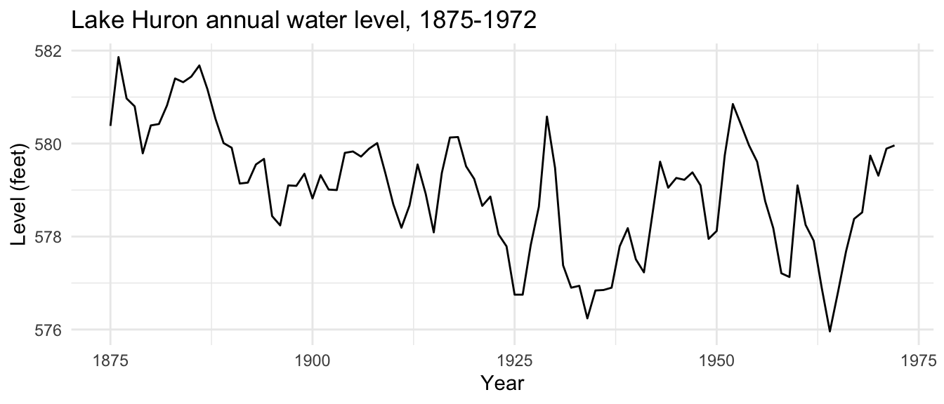

It drifts downward and meanders on the way. Is that a deterministic trend, a stochastic one, or just a persistent stationary series that happens to wander within this window? Let’s ask the tests.

Code

adf.test(LakeHuron)


    Augmented Dickey-Fuller Test

data:  LakeHuron
Dickey-Fuller = -2.7796, Lag order = 4, p-value = 0.254
alternative hypothesis: stationary

Code

kpss.test(LakeHuron)


    KPSS Test for Level Stationarity

data:  LakeHuron
KPSS Level = 0.99529, Truncation lag parameter = 3, p-value = 0.01

ADF cannot reject a unit root, and KPSS rejects stationarity. Both point the same way: as it stands, this series is not stationary. So we difference and check.

Code

lakeHuronDiff <- diff(LakeHuron)
adf.test(lakeHuronDiff)


    Augmented Dickey-Fuller Test

data:  lakeHuronDiff
Dickey-Fuller = -5.4687, Lag order = 4, p-value = 0.01
alternative hypothesis: stationary

Code

kpss.test(lakeHuronDiff)


    KPSS Test for Level Stationarity

data:  lakeHuronDiff
KPSS Level = 0.060391, Truncation lag parameter = 3, p-value = 0.1

The differenced series clears both tests. lakeHuronDiff is stationary, same as the planted walk once we differenced it.

A test is a tool, not an oracle, and Lake Huron is a good place to see why. ADF is known to have low power: it struggles to tell a true unit root from a stationary series with a coefficient close to one, and Lake Huron is well-described as a stationary AR(2) with strong persistence. A lake also has a physical floor and ceiling; the water level cannot wander off to infinity the way a true random walk can, so a literal unit root is implausible on mechanistic grounds no matter what the test prints. So do not read the result as a verdict. Read it as a narrowed question: the data are persistent enough that ADF cannot rule out a unit root, and that persistence is the thing I have to handle either way. The p-value narrows the question but can’t answer it. Mechanism can.

It is also worth watching the tests clear a series, so we do not leave thinking everything is a hidden random walk. Return to the stationary AR(1) from the start of the chapter, the calm top-left panel where the others all misbehaved. We called it stationary and moved on without testing it. Now we can hold it to the same standard.

Code

adf.test(stationarySeries)


    Augmented Dickey-Fuller Test

data:  stationarySeries
Dickey-Fuller = -6.3943, Lag order = 6, p-value = 0.01
alternative hypothesis: stationary

Code

kpss.test(stationarySeries)


    KPSS Test for Level Stationarity

data:  stationarySeries
KPSS Level = 0.076328, Truncation lag parameter = 5, p-value = 0.1

ADF rejects the unit root and KPSS does not reject stationarity, so the series is stationary, which is what we built it to be. The tools do not simply cry “unit root” at everything. They pass a series that has earned the assumption and flag one that has not. Plenty of measured series pass on the first try with no differencing at all, and the exercises put a few from earlier chapters through the same workflow so you can see both outcomes for yourself.

Wrapping Up

Stationarity is the condition under which the rest of our tools are licensed to work. A stationary series keeps a constant mean, a constant variance, and an autocovariance that depends only on the lag. The canonical way that fails is the unit root, the \(\phi = 1\) random walk, where shocks accumulate instead of fading and the variance grows without bound.

The distinction that matters most in practice is between a deterministic trend, which you detrend, and a stochastic trend, which you difference. They can look identical on a plot, the repairs are not interchangeable, and getting it wrong either leaves the problem in place or invents a new one. ADF and KPSS, read together and against what you know about the mechanism, are how you decide.

That decision is the missing piece of the modeling story we started two chapters ago. We can fit AR and MA models, but only to stationary data. When a series is not stationary, we difference it first and then fit ARMA to what is left. Difference, then model: that is the whole idea behind ARIMA, and it is where we go next.

Exercises

Tell the twins apart

The two-kinds-of-trend section built a deterministic-trend series and a stochastic-trend series that looked alike. This time you will be handed the series without the labels and have to classify them.

Code

set.seed(101)
n <- 250
t <- 1:n
mysteryA <- 0.04 * t + arima.sim(list(ar = 0.5), n = n)
mysteryB <- cumsum(rnorm(n)) + 0.04 * t

Plot both. Can you tell which is trend-stationary and which is difference-stationary by eye? Say how confident you are.
Run ADF and KPSS on each. What do the two tests say about each series?
Apply the correct repair to each (detrend one, difference the other), and confirm with the tests that your repaired series is stationary. Then apply the wrong repair to each and describe what goes wrong.

Overdifferencing

We claimed that differencing a series that did not need it injects a spurious moving-average wobble. Show it. Take a stationary AR(1) series, difference it once, and look at the ACF and PACF of the result. The lag-1 autocorrelation of the differenced series will go negative. Where did that come from, given that the original series had none? This is the cost of differencing when you should have left the series alone.

Test a series you have already met

Pick a series from an earlier chapter (the Nile flow, the nhtemp temperatures, or the co2 record from the intro) and run the full workflow on it: plot it, run ADF and KPSS, decide whether it needs differencing, and if it does, difference it and confirm the result clears the tests. For whichever series you choose, write a sentence on whether a unit root is plausible mechanistically, the way we argued about Lake Huron, or whether the apparent trend is more likely deterministic.

Big Idea

Packages

What Stationarity Means

When \(\phi = 1\): the Random Walk

Two Kinds of Trend

Testing for a Unit Root: ADF and KPSS

An Observed Series: Lake Huron

Wrapping Up

Exercises

Tell the twins apart

Overdifferencing

Test a series you have already met

Further Reading