Aside: Detecting a Breakpoint

Introduction

Mann-Kendall and Theil-Sen, from the last chapter, both assume the same shape of change: a gradual, one-directional drift that runs the whole length of the record. That’s a fair assumption for a warming climate or a shrinking snowpack. It’s a bad assumption for a river below a new dam, a gauge that got moved, a lake after its sewage outflow was diverted, or a monitoring program that switched instruments halfway through. None of those series drift. They sit at one level, something happens, and they sit at a new level. If you hand a step change to Mann-Kendall it will usually find something (we’ll watch it do exactly that below), but the number it reports describes a drift that never happened.

What you actually want to ask is different: is there a single moment where the series stopped being one thing and became another, and if so, when? Eyeballing a plot and squinting at the year things look different is not that answer, it’s a guess dressed up as an observation. This aside builds the tool that replaces the squint: find the split point that best separates a series into a before and an after, and test whether that split is worth believing at all.

Packages

The idea here is simple enough to build from scratch, and we will, once. For anything past a single break, or for a proper test of whether a break is there at all, strucchange (Zeileis et al. 2024) does the work. It isn’t used anywhere else in the book, so consider this its one appearance.

library(strucchange)

A Series That Steps Instead of Slides

Plant a series with a single clean jump in it: forty-five points at a mean of 10, then thirty-five points at a mean of 15, both with the same noise.

set.seed(21)
n <- 80
step <- c(rnorm(45, mean = 10, sd = 2), rnorm(35, mean = 15, sd = 2))

tibble(t = 1:n, x = step) |>
  ggplot(aes(t, x)) +
  geom_line(color = bookPal[1]) +
  geom_vline(xintercept = 45.5, linetype = "dashed", color = bookPal[5]) +
  labs(x = "Time", y = "Some variable", title = "A step, not a slope") +
  theme_minimal()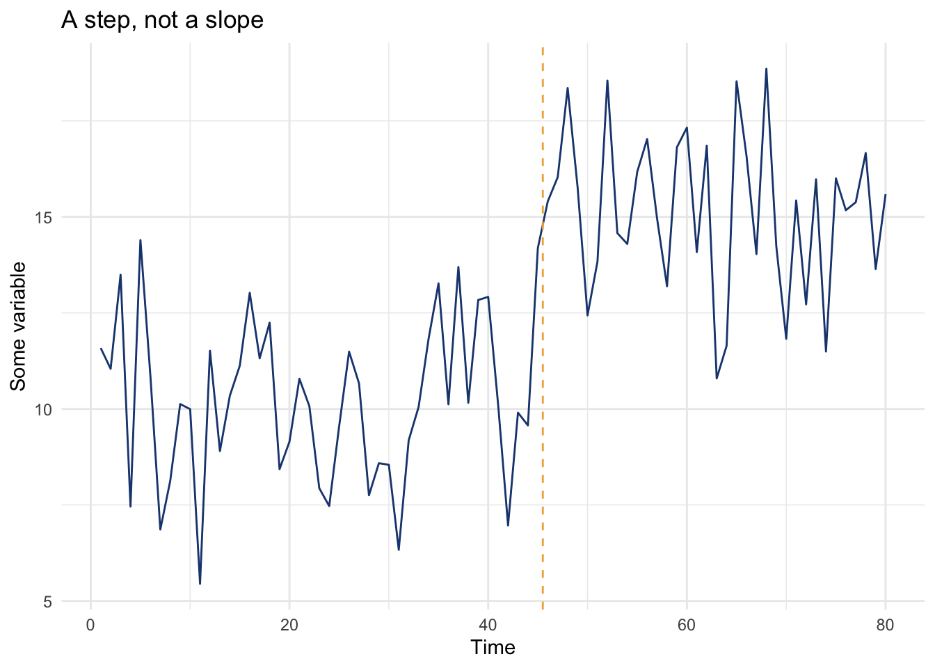

Nothing drifts here. The series is flat, jumps once, and is flat again. Run last chapter’s tools on it anyway.

mannKendall <- function(x) {
  n <- length(x)
  S <- 0
  for (j in 2:n) {
    for (i in 1:(j - 1)) {
      S <- S + sign(x[j] - x[i])
    }
  }
  ties <- table(x)
  tieTerm <- sum(ties * (ties - 1) * (2 * ties + 5))
  varS <- (n * (n - 1) * (2 * n + 5) - tieTerm) / 18
  Z <- (S - sign(S)) / sqrt(varS)
  tau <- S / (n * (n - 1) / 2)
  p <- 2 * (1 - pnorm(abs(Z)))
  tibble(S = S, varS = varS, Z = Z, tau = tau, p = p)
}

theilSen <- function(x, t = seq_along(x)) {
  n <- length(x)
  slopes <- c()
  for (j in 2:n) {
    for (i in 1:(j - 1)) {
      slopes <- c(slopes, (x[j] - x[i]) / (t[j] - t[i]))
    }
  }
  median(slopes)
}

mkStep <- mannKendall(step)
tsStep <- theilSen(step)
c(tau = mkStep$tau, p = mkStep$p, theilSenPerUnit = tsStep)

            tau               p theilSenPerUnit 
   4.373418e-01    9.603393e-09    9.030074e-02 

Mann-Kendall reports \(\tau\) = 0.44 with a \(p\)-value of 9.6e-09. Screaming significant, as it should be, later values really do sit above earlier ones. The Theil-Sen slope of 0.09 per unit time, multiplied out over 79 points, lands close to the actual jump of 5. But look at what that slope claims: a steady climb, a little bit every year, for eighty years. That’s not what happened. Nothing moved for forty-five points, then five units of change arrived at once, then nothing moved again. The number is roughly the right size and describes the wrong process entirely. Wrong tool for this shape of change, even when it doesn’t look wrong.

Finding the Break by Hand

Here’s the idea, and it is about as simple as Mann-Kendall’s pairwise sum. Try every possible split point. At each one, take the mean of everything before it and the mean of everything after, and add up how far every point sits from its own segment’s mean. That leftover variation, the residual sum of squares, is small when the split falls right where the series actually changes and large everywhere else. The split that minimizes it is your best guess at the breakpoint.

rssAtSplit <- function(x, k) {
  before <- x[1:k]
  after <- x[(k + 1):length(x)]
  sum((before - mean(before))^2) + sum((after - mean(after))^2)
}

candidates <- 5:(n - 5)
rss <- map_dbl(candidates, rssAtSplit, x = step)
bestSplit <- candidates[which.min(rss)]
bestSplit

[1] 44

tibble(split = candidates, rss = rss) |>
  ggplot(aes(split, rss)) +
  geom_line(color = bookPal[1]) +
  geom_vline(xintercept = bestSplit, linetype = "dashed", color = bookPal[5]) +
  labs(x = "Candidate split point", y = "Leftover variation (RSS)",
    title = "Where the series is best explained by two means instead of one") +
  theme_minimal()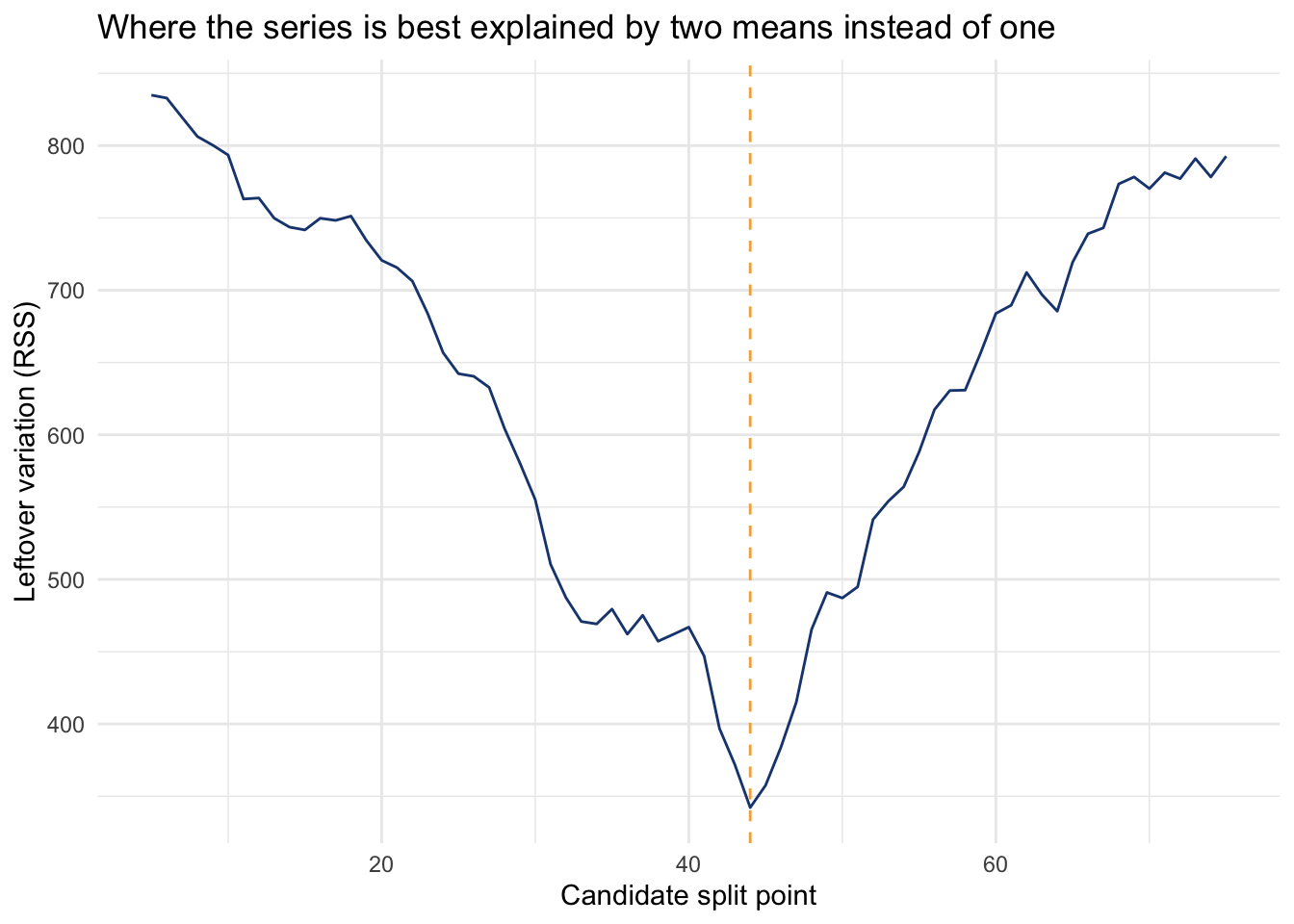

The minimum lands at point 44, one point off the true break at 45, about as close as noisy data lets you get. Compare that RSS at the best split, 342.2, against the RSS if you’d insisted on a single mean for the whole series, 838.1. Cutting the series in two explains a lot more of it. That comparison, one mean’s leftover variance against two means’ leftover variance, is exactly what an F-test asks. This by-hand scan is a Chow test with extra steps.

A Formal Test: strucchange

strucchange::breakpoints() runs the same search, more carefully. Instead of one split, it solves for the best partition at every number of breaks and lets BIC pick how many are actually worth keeping.

bpStep <- breakpoints(step ~ 1)
bpStep$breakpoints

[1] 44

Same answer as the by-hand scan, point 44, because for one break they are the same calculation. What the package adds is a formal test for whether that break should be trusted at all, using the same F-statistic under the hood.

fsStep <- Fstats(step ~ 1)
sctest(fsStep, type = "supF")

    supF test

data:  fsStep
sup.F = 113.04, p-value < 2.2e-16

And a confidence interval on the date itself, not just a point guess.

confint(bpStep)

     Confidence intervals for breakpoints
     of optimal 2-segment partition: 

Call:
confint.breakpointsfull(object = bpStep)

Breakpoints at observation number:
  2.5 % breakpoints 97.5 %
1    42          44     46

Corresponding to breakdates:
  2.5 % breakpoints 97.5 %
1 0.525        0.55  0.575

For the planted series that interval is tight, a couple of points either side of 44, because the jump is large and the noise is modest. Field data is rarely this cooperative, and the interval is where you’ll feel that. The dynamic-programming search behind all of this, extending cleanly from one break to several, is Bai and Perron (2003); the testing-and-dating framing used here, existence first, date second, follows Zeileis et al. (2003).

Autocorrelation Fools This Test Too

Mann-Kendall’s problem, from the last chapter, was autocorrelation: feed it a flat AR(1) series with no trend at all and it cries trend anyway, more often as \(\phi\) climbs. Does a break test fall into the same trap? Run the same kind of check, an AR(1) series with no break in it, and see how often sctest declares one anyway.

ar1Series <- function(phi, n) {
  if (phi == 0) rnorm(n) else as.numeric(arima.sim(list(ar = phi), n = n))
}

bpFalsePositive <- function(phi, n = 60, sims = 200) {
  mean(replicate(sims, {
    fs <- Fstats(ar1Series(phi, n) ~ 1)
    sctest(fs, type = "supF")$p.value < 0.05
  }))
}

set.seed(10)
phis <- c(0, 0.3, 0.5, 0.7, 0.9)
bpFp <- tibble(phi = phis, rate = map_dbl(phis, bpFalsePositive))
bpFp

# A tibble: 5 × 2
    phi  rate
  <dbl> <dbl>
1   0   0.065
2   0.3 0.255
3   0.5 0.425
4   0.7 0.765
5   0.9 0.93 

ggplot(bpFp, aes(factor(phi), rate)) +
  geom_col(fill = bookPal[5], width = 0.6) +
  geom_hline(yintercept = 0.05, linetype = "dashed") +
  scale_y_continuous(labels = scales::percent) +
  labs(x = expression("AR(1) coefficient " * (phi)),
    y = "Breaks declared significant",
    title = "A break test finds a break in break-free data too",
    subtitle = "Share of 200 flat AR(1) series called significant at the 5% level") +
  theme_minimal()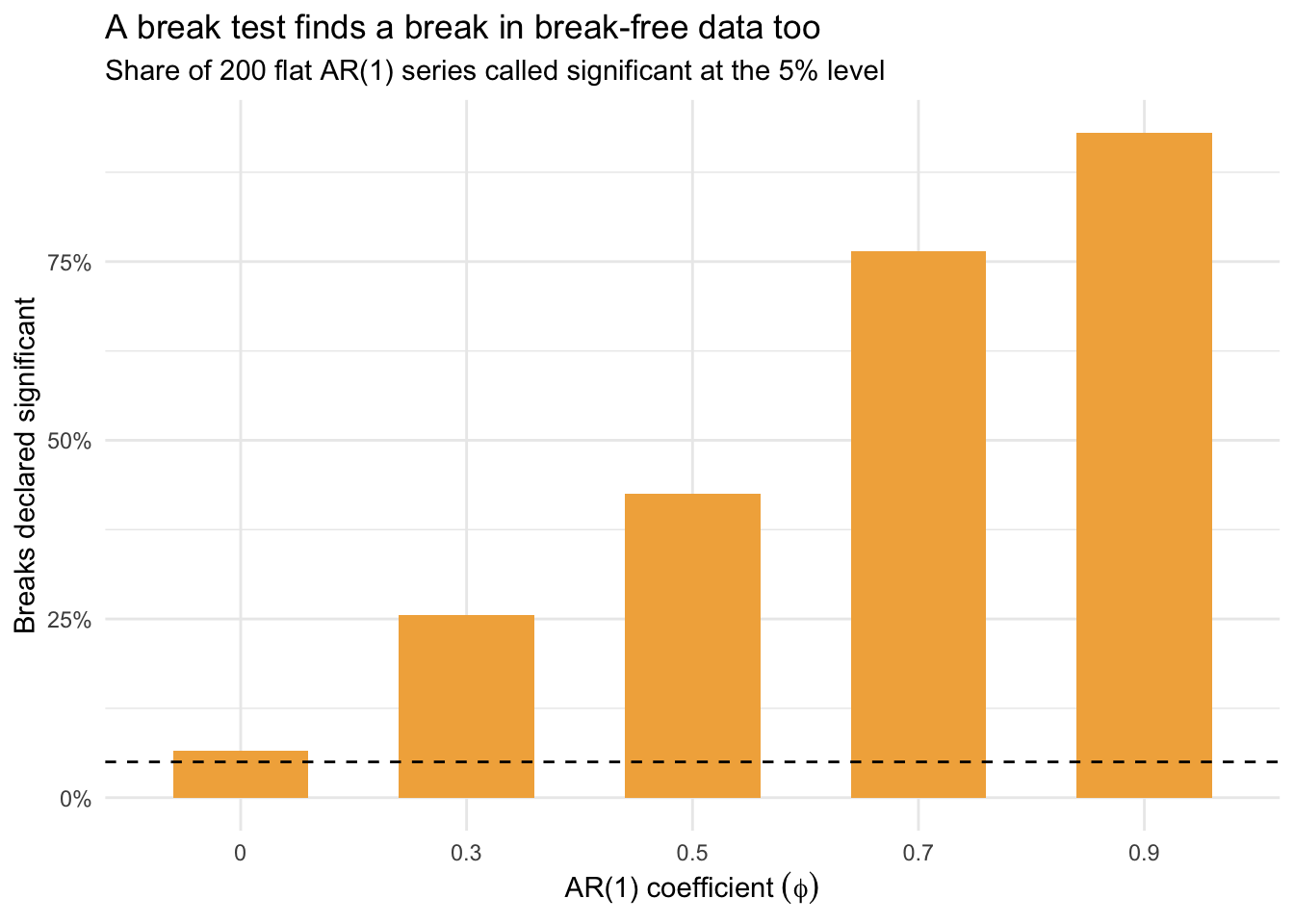

Same trap, different shape of test. At \(\phi = 0\) the false-positive rate sits close to the nominal 5%. By \(\phi = 0.9\) it’s declaring a break in most series that never had one. A run of correlated years looks, to an F-test built for independent noise, exactly like the kind of level shift it was built to catch. There is a fix, the same family of fix as GLS in the regression chapter: replace the test’s covariance estimate with one that accounts for the autocorrelation instead of assuming it away (Zeileis et al. 2003). Building that correctly is more than this aside has room for, so take the caution as the headline: a breakpoint test run on a dependent series is just as capable of finding a break that isn’t there as Mann-Kendall was of finding a trend that wasn’t.

An Observed Series: the Nile, Again

The autocorrelation chapter introduced the Nile’s annual flow at Aswan and pointed out a visible drop around the turn of the century, marked it as the Aswan Low Dam, under construction from 1898 and finished in 1902, and moved on, calling it a known break so it wouldn’t distract from the autocorrelation question at hand. This is where we come back for it. Set the history aside for a moment: if all you had was the series, could you find that break on your own, and how sure could you be of the year?

data(Nile)
bpNile <- breakpoints(Nile ~ 1)
bpNile$breakpoints

[1] 28

nileBreakYear <- time(Nile)[bpNile$breakpoints]
nileCI <- confint(bpNile)
nileCIYears <- time(Nile)[nileCI$confint]
nileBefore <- mean(Nile[1:bpNile$breakpoints])
nileAfter <- mean(Nile[(bpNile$breakpoints + 1):length(Nile)])

c(breakYear = nileBreakYear, before = round(nileBefore, 1), after = round(nileAfter, 1))

breakYear    before     after 
   1898.0    1097.8     850.0 

tibble(year = as.numeric(time(Nile)), flow = as.numeric(Nile)) |>
  ggplot(aes(year, flow)) +
  geom_line(color = bookPal[1]) +
  geom_vline(xintercept = nileBreakYear, linetype = "dashed", color = bookPal[5]) +
  annotate("rect", xmin = nileCIYears[1], xmax = nileCIYears[2], ymin = -Inf, ymax = Inf,
    fill = bookPal[5], alpha = 0.1) +
  labs(x = "Year", y = expression(10^8 ~ m^3),
    title = "River Nile, annual flow: best single break",
    subtitle = "Shaded band is the 95% confidence interval on the break date") +
  theme_minimal()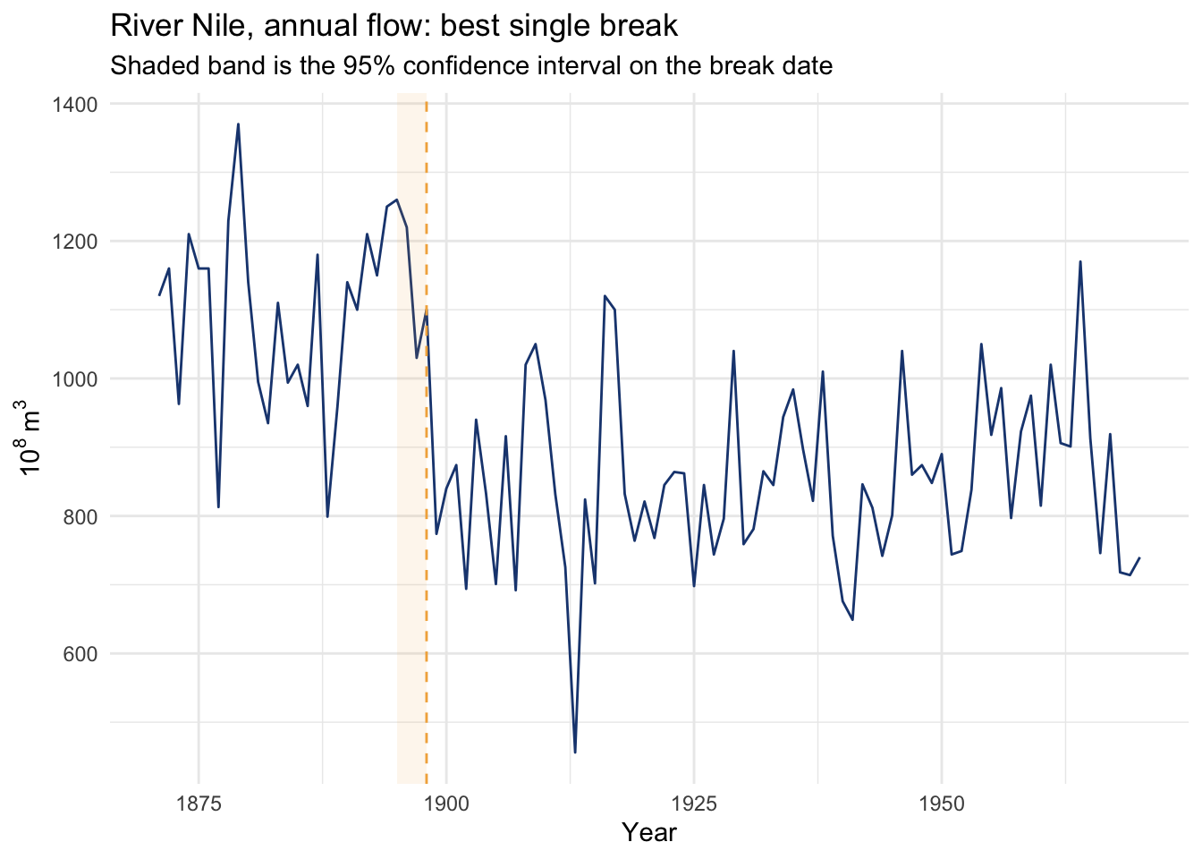

The break lands at 1898, the year the dam’s construction began, and the mean drops from 1097.8 to 850, about 247.8 (units of \(10^8\) m\(^3\)) lower on average once the dam started holding water back. The 95% confidence interval, 1895 to 1898, brackets almost exactly the span from the start of construction to its completion. And the existence test isn’t shy about it either.

fsNile <- Fstats(Nile ~ 1)
sctest(fsNile, type = "supF")

    supF test

data:  fsNile
sup.F = 75.93, p-value = 2.22e-16

That’s what a break test looks like when the premise actually holds: one structural cause, one clean jump in the mean, and a date narrow enough to match the history books without having read them first. The planted step earlier in this aside was built to behave exactly this well. Most series aren’t this obliging, which is worth remembering the next time a break test hands you a tight interval on something you can’t independently check.

Where This Shows Up

The Nile had its answer waiting in the history books. Most series won’t. A detected break is a hypothesis about a date, not an explanation, and before you trust one, go find out what actually happened around that year, a gauge relocation, a dam, a change in land use, a new instrument. Sometimes there’s a clean answer. Sometimes there isn’t, and the plain move is to say the series shifted and you don’t know why. Either way, a breakpoint test and a trend test are asking different questions about the same word, “change,” and a series that fails one can still fail the other. Run both, and let the data tell you which shape it actually took.