Aside: Filling a Gap With a Neighbor

Introduction

Every long-running weather station has a story about the years it wasn’t running: a sensor failed, a funding line dried up, an airport moved its equipment and nobody thought to keep the old site going in parallel. The Bellingham airport station this book keeps coming back to (kbli) has one too. Its full 1949-to-present monthly record has a 27-month hole, July 1996 through September 1998, that shows up plainly as NA in data/kbli_monthly.csv rather than being papered over.

A short gap in something that barely changes from one reading to the next (an hourly radiation sensor, say) can be patched by interpolating between its own neighbors, which is exactly what the filters chapter did with na.approx() and na.spline(). A 27-month hole in monthly temperature is a different problem: there is no straight line across two years that has any business standing in for two years of actual winters and summers. When the gap is that long, the fix people actually reach for in climate and weather work is not to look harder at the gappy station, it’s to borrow information from a different station nearby that kept reporting the whole time.

Packages

We stay with tidyverse (Wickham 2023) for wrangling and plotting and PNWColors (Lawlor 2020) for the figure colors.

library(tidyverse)
library(PNWColors)

bookPal <- pnw_palette("Sunset2", n = 5, type = "discrete")

A Station Three Miles Away

USC00450587, known in NOAA’s records as Bellingham 3 SSW, sits about three miles south-southwest of the airport and is part of the Historical Climatology Network, one of NOAA’s longer and more carefully maintained station sets. It was running the whole time the airport gauge went dark. data/bellingham_3ssw_temp.csv holds its monthly mean temperature, derived from daily TMAX/TMIN the same way kbli’s is.

kbli <- read_csv("data/kbli_monthly.csv")
donor <- read_csv("data/bellingham_3ssw_temp.csv") |> rename(donorTavg = TAVG)

full_join(kbli, donor, by = "DATE") |>
  filter(DATE >= as.Date("1993-01-01"), DATE <= as.Date("2001-12-01")) |>
  pivot_longer(c(TAVG, donorTavg), names_to = "series", values_to = "tavg") |>
  mutate(series = recode(series,
    TAVG = "Bellingham Airport (kbli)",
    donorTavg = "Bellingham 3 SSW (donor)"
  )) |>
  ggplot(aes(DATE, tavg, color = series)) +
  geom_line() +
  scale_color_manual(values = c(
    "Bellingham Airport (kbli)" = bookPal[1],
    "Bellingham 3 SSW (donor)" = bookPal[5]
  )) +
  labs(
    x = NULL, y = expression(degree * C), color = NULL,
    title = "The airport gap, and a station three miles away that kept reporting"
  ) +
  theme_minimal()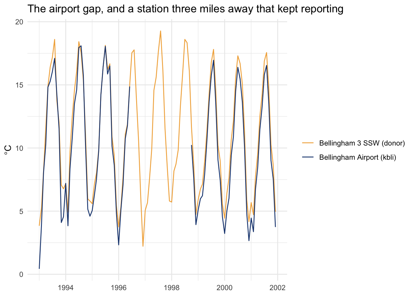

The airport line simply stops in the middle of 1996 and doesn’t pick back up until late 1998. The donor line runs straight through, tracking the same seasonal shape a little warmer year-round, which is what you’d expect from two nearby sites with slightly different exposure and elevation.

Calibrating the Donor

Before the donor station can stand in for the missing months, we need to know exactly how the two relate during the months they both reported.

overlap <- inner_join(kbli, donor, by = "DATE") |> drop_na()
nrow(overlap)

[1] 165

ggplot(overlap, aes(donorTavg, TAVG)) +
  geom_point(color = "grey40", alpha = 0.6) +
  geom_smooth(method = "lm", se = FALSE, color = bookPal[5]) +
  labs(
    x = expression("Bellingham 3 SSW monthly " * degree * C),
    y = expression("Bellingham Airport monthly " * degree * C),
    title = paste(nrow(overlap), "months where both stations reported")
  ) +
  theme_minimal()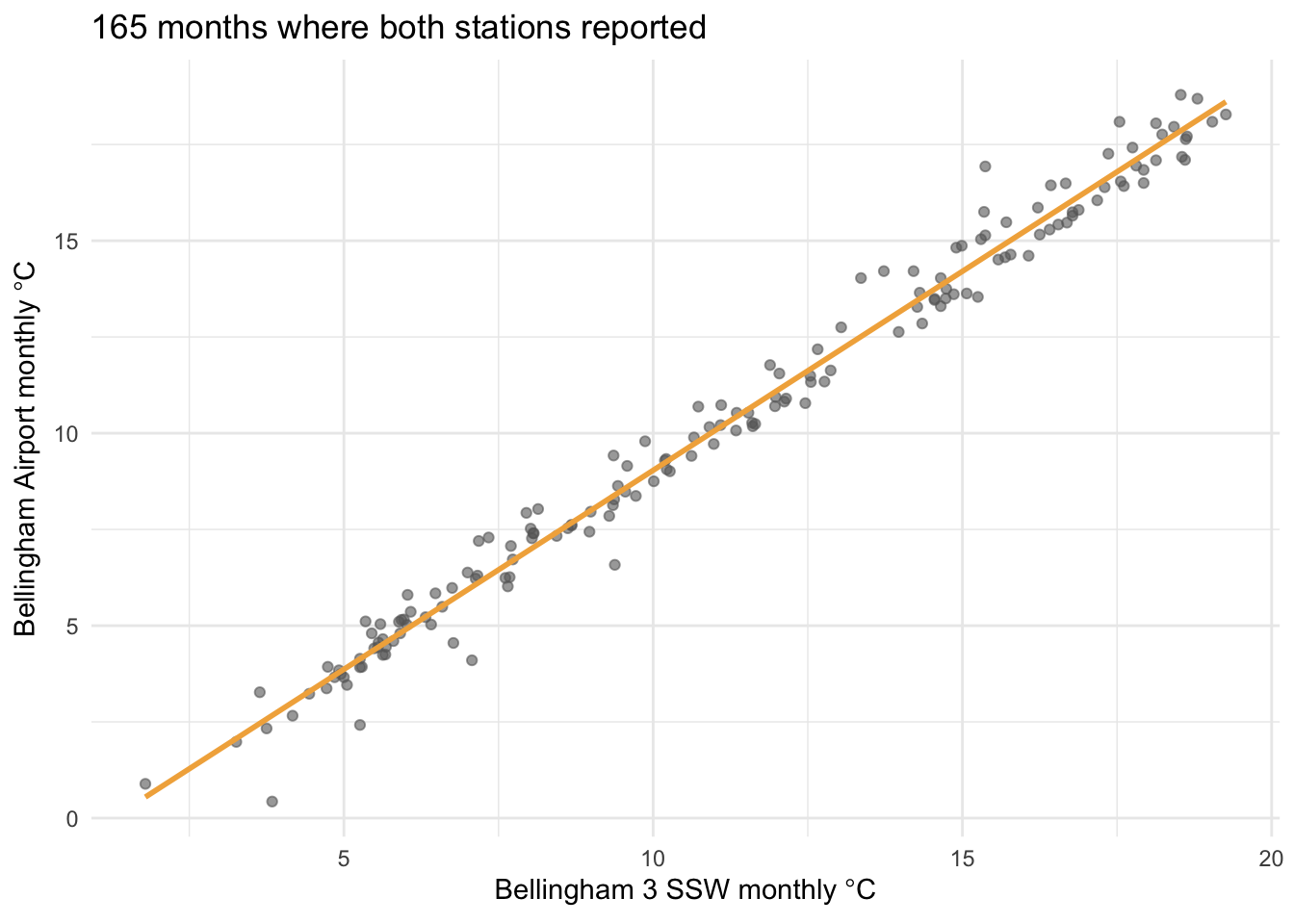

165 months, and the relationship is close to a straight line the whole way from winter lows to summer highs. A simple linear model captures it well.

overlapFit <- lm(TAVG ~ donorTavg, data = overlap)
summary(overlapFit)$r.squared

[1] 0.984201

coef(overlapFit)

(Intercept)   donorTavg 
  -1.303921    1.033950 

An R² of 0.984 and a slope close to 1 (1.03) with a small negative intercept (-1.3): the airport runs a little cooler than the inland donor site, consistently, across the full range of temperatures either station sees.

Does It Actually Work?

A good fit on the months you already have doesn’t automatically mean the donor will do a good job standing in for months you don’t have. Test it the way this book always tests a model before trusting it: hold out a stretch of known months, refit on everything else, predict the held-out stretch from the donor alone, and check the damage.

trainSet <- overlap |> filter(year(DATE) < 2000 | year(DATE) > 2003)
testSet <- overlap |> filter(year(DATE) >= 2000, year(DATE) <= 2003)

validateFit <- lm(TAVG ~ donorTavg, data = trainSet)
testPred <- predict(validateFit, newdata = testSet)
rmseRegression <- sqrt(mean((testPred - testSet$TAVG)^2))

climLookup <- trainSet |>
  mutate(mo = month(DATE)) |>
  group_by(mo) |>
  summarise(climMean = mean(TAVG))
rmseClimatology <- testSet |>
  mutate(mo = month(DATE)) |>
  left_join(climLookup, by = "mo") |>
  summarise(rmse = sqrt(mean((climMean - TAVG)^2))) |>
  pull(rmse)

tibble(
  method = c("donor regression", "climatology baseline"),
  rmseDegC = c(rmseRegression, rmseClimatology)
)

# A tibble: 2 × 2
  method               rmseDegC
  <chr>                   <dbl>
1 donor regression        0.441
2 climatology baseline    1.35 

The withheld stretch is 2000 through 2003, four years nowhere near the actual gap, chosen only because the true values are known and can be checked against. The donor-based regression misses by about 0.44°C on average; a naive baseline that just uses each calendar month’s long-run average misses by about 1.35°C, roughly 3.1 times worse. The donor station is picking up the specific weather in a specific month, not just the season, and that’s exactly the property you want before you let it speak for two years you can’t check.

Filling the Gap

With the technique validated, refit on every month of overlap (more data than the validation split used) and predict the 27 months the airport actually missed.

finalFit <- lm(TAVG ~ donorTavg, data = overlap)

gapFilled <- kbli |>
  filter(is.na(TAVG)) |>
  select(DATE) |>
  inner_join(donor, by = "DATE") |>
  mutate(
    TAVG = predict(finalFit, newdata = tibble(donorTavg = donorTavg)),
    source = "filled"
  )

kbliComplete <- kbli |>
  drop_na() |>
  mutate(source = "measured") |>
  bind_rows(gapFilled) |>
  arrange(DATE)

kbliComplete |>
  filter(DATE >= as.Date("1993-01-01"), DATE <= as.Date("2001-12-01")) |>
  ggplot(aes(DATE, TAVG, color = source)) +
  geom_line(aes(group = 1), color = "grey70") +
  geom_point(size = 1) +
  scale_color_manual(values = c(measured = "grey30", filled = bookPal[5])) +
  labs(
    x = NULL, y = expression(degree * C), color = NULL,
    title = "27 months filled from the donor"
  ) +
  theme_minimal()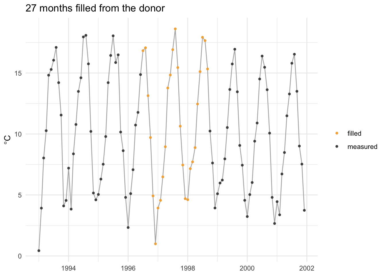

kbliComplete is a new object built just for this aside. It is not a replacement for data/kbli_monthly.csv, and the filters chapter’s version of this record still shows the gap exactly as measured. The point here isn’t that every gap should be filled by default; it’s that when you decide to fill one, the source column above is not decorative: three years from now, whoever reuses this series should be able to tell instantly which 27 points are estimates riding on a neighboring station’s word, not readings off Bellingham’s own instrument.

Closing

This aside used one hand-picked neighbor and a plain linear regression, because that’s enough to show the idea working end to end on an actual 27-month hole. National weather services do a more careful version of the same thing at scale (multiple neighboring stations, formal checks for undocumented station moves and instrument changes, statistical tests for whether the target and donor drift apart over time), all built on the same foundation: find a series that correlates with the one you’re missing, calibrate the relationship on the months you can check, and validate that calibration on more months you can check before you ever apply it to months you can’t.

One thing worth being direct about: this aside only fills temperature. The daily record behind kbli also carries a PRCP column, and a climatologist trying to reconstruct a complete station history would need to close that gap too. Precipitation doesn’t cooperate the way temperature does. Rain and snow fall in patches, a storm can soak one station and miss another three miles away, so two nearby gauges correlate far less tightly than two nearby thermometers do. Precip is also zero-inflated, most months have several days that report exactly zero, which breaks the assumptions behind a plain linear regression like overlapFit. Filling a precipitation gap properly usually calls for something like a generalized linear model built around that zero-inflation, not the two-line lm() this aside got away with for temperature.