Aside: How Ccf Normalizes

Introduction

The eagle-eyed reader will notice that the numbers from Ccf do not line up exactly with what cor gives for the same pair of lagged vectors. They are close, but not identical. This drove me to madness when students would ask me exactly why this was. This aside takes the lid off and shows why. None of it is required to use cross-correlation. It is here for the reader who wants to know what the function is doing under the hood, which matters most when the lags get large, as they did with the algae and the grazers.

library(tidyverse)
library(forecast)
library(PNWColors)

bookPal <- pnw_palette("Sunset2", n = 5, type = "discrete")

The Discrepancy

Let’s build a series where \(y\) depends on \(x\) at lag one, using a zero for the first value so we do not introduce an NA.

n <- 100
x <- rnorm(n)
y <- 0.8 * c(0, x[1:(n - 1)]) + rnorm(n, sd = 0.5)

# the two vectors aligned for lag 1
xLag <- x[1:(n - 1)]
yTrunc <- y[2:n]

Here are the first fifty points of the two series we built.

tibble(time = 1:n, x, y) |>
  filter(time <= 50) |>
  pivot_longer(c(x, y)) |>
  ggplot(aes(time, value, color = name)) +
  geom_line() +
  scale_color_manual(values = c(x = bookPal[1], y = bookPal[5])) +
  labs(x = "Time", y = NULL, color = NULL) +
  theme_minimal()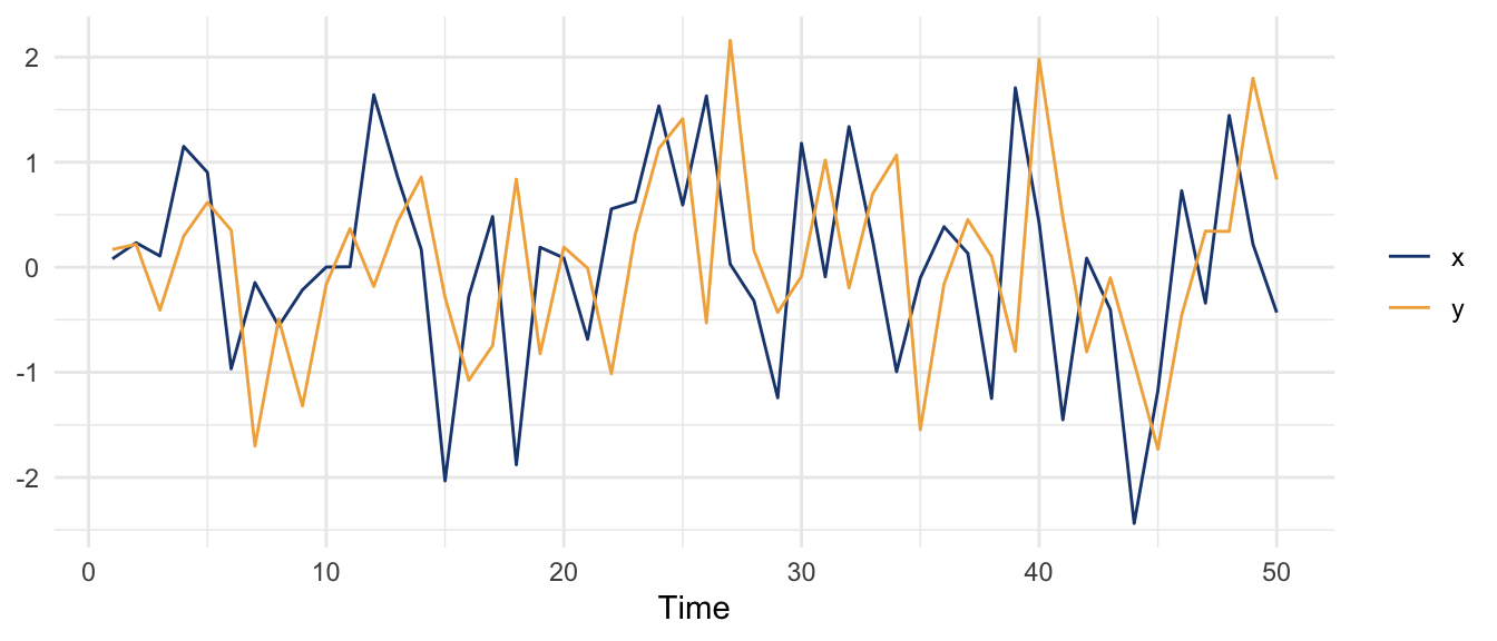

The ordinary Pearson correlation at lag one uses only the overlapping pairs, all \(n - 1\) of them, and computes its means and standard deviations from that subset.

cor(xLag, yTrunc)

[1] 0.8348397

Now compare that to what Ccf reports at the same lag.

ccfObj <- Ccf(x, y, lag.max = 10, plot = FALSE)
ccfLag1 <- ccfObj$acf[ccfObj$lag == -1]
ccfLag1

[1] 0.8342341

The two numbers are very close but slightly different. The reason is that Ccf, like Acf, normalizes every lag against the full series rather than the overlapping subset. It uses only the \(n - 1\) available pairs in the numerator, but it divides by standard deviations computed from all \(n\) values of each series. The same denominator is used at every lag, no matter how many pairs actually overlap.

Reproducing It by Hand

We can rebuild the Ccf value at lag one from its parts. The numerator is the cross-product of the lagged pairs around the full-series means; the denominator is the full-series standard deviations scaled by the number of pairs.

k <- 1
num   <- sum((xLag - mean(x)) * (yTrunc - mean(y)))  # full-series means
denom <- (n - k) * sd(x) * sd(y)                        # full-series sds
num / denom

[1] 0.8342341

That matches ccfLag1 exactly.

So why hold the denominator fixed? Because it puts every lag on the same footing. As the lag grows the number of overlapping pairs shrinks, and if you let each lag normalize against its own dwindling subset, the correlations at far lags would be scaled differently from the ones near zero and you could not compare them on a single plot. Anchoring the standard deviations to the whole series keeps the whole cross-correlation function on one scale. It is a small thing, and it almost never changes a conclusion, but when you are reading a lead off a plot at a lag of forty days, as we did with the producers and grazers, it is worth knowing that the function has been holding the scale steady for you.

Now you know.