Aside: The PACF by Hand

Introduction

In the autocorrelation chapter we used Pacf to read the partial autocorrelation off a plot and never asked how the number got there. The short version was that the partial autocorrelation at lag \(k\) is the correlation between \(y_t\) and \(y_{t-k}\) after the intervening lags have been accounted for. This aside takes the lid off and shows you that the partial autocorrelation is nothing more exotic than a regression coefficient, computed lag by lag. None of it is required to use the PACF. It is here for the reader who wants to see that the function is not doing anything magic.

We need a series to work with. Let’s build the same kind of AR(1) we used in the chapter, so the answers line up with what you have already seen.

library(forecast)
n <- 500
phi <- 0.7
epsilon <- rnorm(n)
y <- numeric(n)
for (i in 2:n) y[i] <- phi * y[i - 1] + epsilon[i]

Warming Up: the ACF by Hand

Before the partial version, let’s confirm we can reproduce the plain ACF ourselves, because the PACF builds on it. The autocorrelation at a lag is just the ordinary correlation between the series and a shifted copy of itself. Compare the values Acf reports at lags 1 and 2 to what cor gives when we line up the series against its own lags.

yACF <- Acf(y, plot = FALSE)
# ACF for lag 1 and lag 2, straight from Acf
round(yACF$acf[2, , ], 2)

[1] 0.67

round(yACF$acf[3, , ], 2)

[1] 0.39

# the same thing, done by hand with cor
yLag1 <- c(y[-1], NA)
yLag2 <- c(y[-c(1, 2)], NA, NA)
round(cor(yLag1, y, use = "complete.obs"), 2)

[1] 0.67

round(cor(yLag2, y, use = "complete.obs"), 2)

[1] 0.4

The values differ a little past the second decimal because cor and Acf divide by slightly different degrees of freedom, but they are the same quantity. We can wrap the idea in a loop and rebuild the whole correlogram.

yACFv2 <- numeric(25)
for (i in 1:25) {
  yLag <- y[-(1:i)]
  yClip <- y[1:length(yLag)]
  yACFv2[i] <- cor(yClip, yLag)
}

par(mfcol = c(1, 2))
Acf(y, ylim = c(-0.1, 0.8), main = "ACF via Acf()")
plot(1:25, yACFv2, type = "h", ylim = c(-0.1, 0.8),
  main = "ACF by hand", xlab = "Lag", ylab = "ACF")
abline(h = 0)
cis <- qnorm((1 + 0.95) / 2) / sqrt(n)
abline(h = c(-cis, cis), lty = "dashed", col = "blue")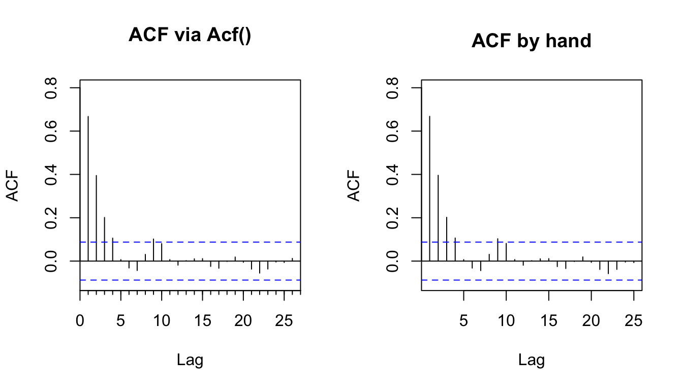

The PACF as a Regression Coefficient

Now the partial version. The trick is to stop using cor and start using lm, fitting through the origin. The partial autocorrelation at lag \(k\) is the coefficient on the lag-\(k\) term in a regression of \(y\) on all of its lags up to \(k\). At lag 1 that is a one-predictor regression. At lag 2 we add the second lag and read the coefficient on it, which measures the effect of \(y_{t-2}\) after the effect of \(y_{t-1}\) has been removed.

yPACF <- Pacf(y, plot = FALSE)
# PACF coefs for lag 1 and lag 2, from Pacf
round(yPACF$acf[1, , ], 2)

[1] 0.67

round(yPACF$acf[2, , ], 2)

[1] -0.09

# the same coefs, from regressions through the origin
round(coef(lm(y ~ yLag1 - 1))[1], 2)

yLag1 
 0.67 

round(coef(lm(y ~ yLag1 + yLag2 - 1))[2], 2)

yLag2 
-0.09 

The lag-1 partial matches the regression coefficient on a single lag, and the lag-2 partial matches the coefficient on the second lag once the first is in the model. To rebuild the whole PACF plot we just keep going, adding one lag at a time and reading the coefficient on the newest lag. That means assembling a matrix of lagged predictors that grows by a column each step.

yPACFv2 <- numeric(25)
for (j in 2:25) {
  nRows <- length(y) - j + 1
  yLagMat <- matrix(0, nRows, j)
  for (i in 1:j) {
    yLagMat[, i] <- y[i:(i + nRows - 1)]
  }
  lm1 <- lm(yLagMat[, 1] ~ yLagMat[, -1] - 1)
  yPACFv2[j] <- coef(lm1)[j - 1]
}

par(mfcol = c(1, 2))
Pacf(y, ylim = c(-0.1, 0.8), main = "PACF via Pacf()")
plot(1:25, yPACFv2, type = "h", ylim = c(-0.1, 0.8),
  main = "PACF by hand", xlab = "Lag", ylab = "PACF")
abline(h = 0)
abline(h = c(-cis, cis), lty = "dashed", col = "blue")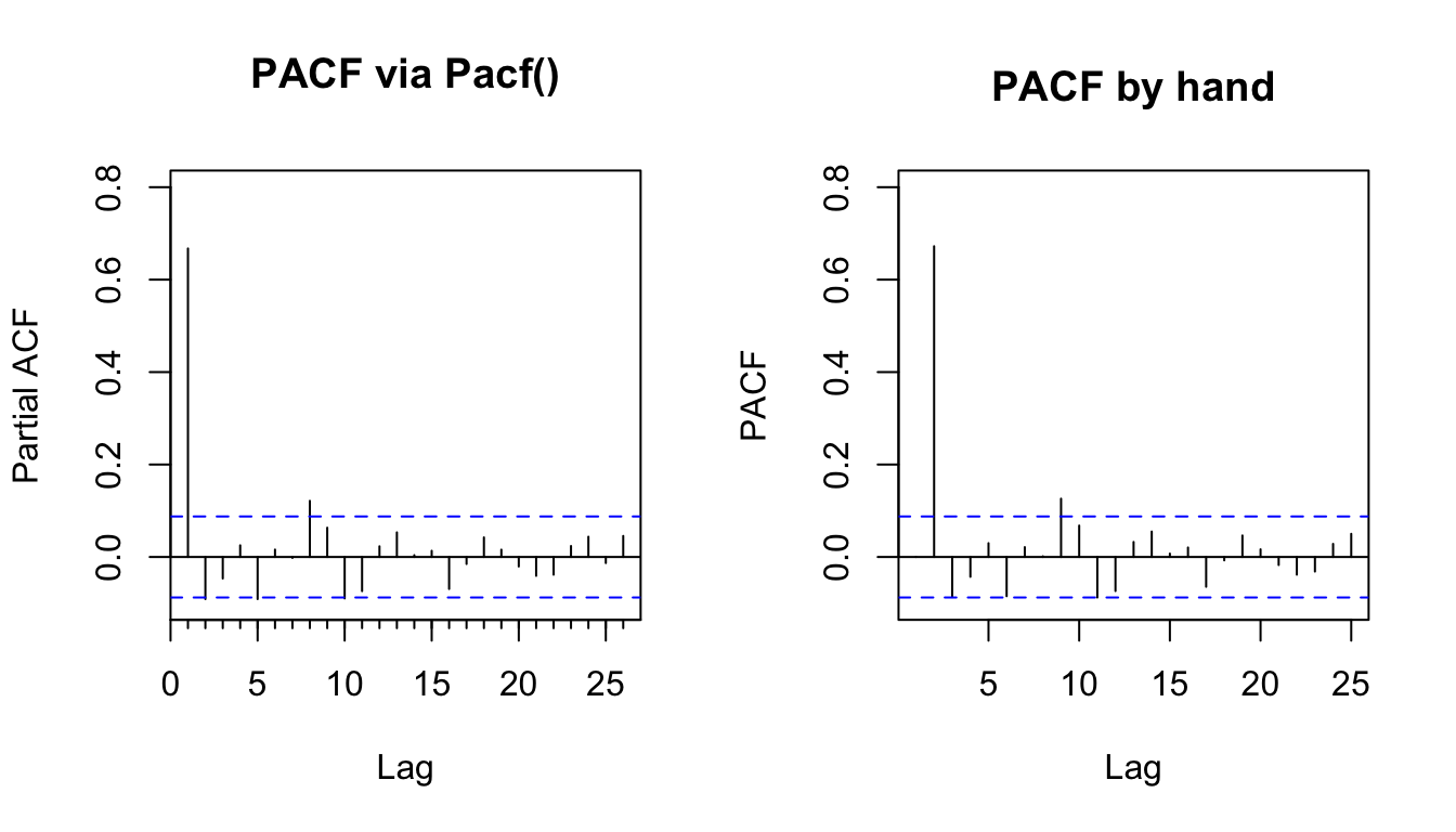

The hand-built version reproduces the spike at lag 1 and the collapse to near zero afterward, which is the AR(1) signature: one strong partial, then nothing.

The Way the Function Actually Does It

Fitting a fresh regression at every lag is fine for understanding but wasteful in practice. The actual pacf function never calls lm. It solves the same system with linear algebra, through what is called the Durbin-Levinson recursion, which turns the autocorrelations directly into partials by solving a Toeplitz system at each order. The details are past where we usually go, but it is satisfying to see that the same numbers fall out.

yACFcoef <- yACF$acf[, , 1]
yPACFv3 <- numeric(26)
for (i in 1:26) {
  yPACFv3[i] <- solve(toeplitz(yACFcoef[1:i]), yACFcoef[2:(i + 1)])[i]
}
round(yPACFv3[1:8], 3)        # PACF by hand, version 3

[1]  0.667 -0.091 -0.047  0.025 -0.091  0.016 -0.002  0.121

round(yPACF$acf[1:8, , 1], 3) # and straight from Pacf

[1]  0.667 -0.091 -0.047  0.025 -0.091  0.016 -0.002  0.121

Same answers, three different ways: a stack of regressions, a growing design matrix, and a Toeplitz solve. The function picks the fast one. You now know what it is computing, which is the only point of the exercise.

Where This Shows Up

Back in the chapter, the rule of thumb was that an AR(p) process shows a sharp PACF cutoff after lag \(p\) while an MA process shows a slow PACF decay. That rule is exactly this regression logic at work: once you have conditioned on enough lags to capture an AR(p) process, the next coefficient has nothing left to explain and drops to zero. When you read a PACF plot to pick the order of a model, this is the machinery you are leaning on.