Reconstruction

Big Idea

Every chapter in this section of the book has fit a model and done something with it. We found the lag at which one series leads another, estimated a slope, tested a trend, and forecast a series forward. We know all models are wrong, right? But we’ve been asking is the model useful? A model can fit the data it was built from beautifully and still be useless on anything else, because fitting and predicting are different acts. The only way to tell them apart is to hold some data back, build the model without it, and see whether the model can predict what it was never shown. That is out-of-sample validation.

This chapter makes that idea concrete by reconstructing the flow of the Colorado River back more than a thousand years from tree rings. We have a short instrumental record of flow and a long proxy that tracks it, we calibrate the relationship where the two overlap, we verify it on years the calibration never saw, and only then do we trust it to reach back before the gauges existed. The tree rings are the worked example. The transferable skill is the validation: the same split-sample check that tells a paleoclimatologist whether a reconstruction is sound is what tells you whether a load forecast or a calibration curve or any predictive model will hold up.

Packages

We hand-build the skill scores, fit the model with base R’s lm, and use the tidyverse (Wickham 2023) for wrangling and plotting. slider (Vaughan 2025) gives us a clean centered running mean and PNWColors (Lawlor 2020) the palette. forecast (Hyndman et al. 2026) gives us ggAcf to check the model’s residuals, nlme (Pinheiro et al. 2026) gives us gls to confirm what that check shows, and tseries (Trapletti and Hornik 2026) gives us adf.test/kpss.test, the same stationarity check from chapter four, to confirm the reconstruction itself.

library(tidyverse)
library(slider)
library(forecast)
library(nlme)
library(tseries)
library(PNWColors)

bookPal <- pnw_palette("Sunset2", n = 5, type = "discrete")

A Short Record and a Long Proxy

The data are the Meko reconstruction of water-year flow for the Colorado River at Lees Ferry (Meko et al. 2007). Dave Meko built it with Connie Woodhouse, the same Woodhouse behind the precipitation-and-flow model we leaned on in the regression chapter (Woodhouse et al. 2016); the two of them have been reconstructing Colorado River flow together for decades, and Woodhouse et al. (2006) is their fuller writeup of the calibration-and-verification method this chapter walks through. They are both legends in the paleo world.

There are two columns. ObsMAF is the observed flow in millions of acre-feet, which exists only for the instrumental period, 1906 to 2004. Millions of acre-feet is on s list of worst units ever but it’s what managers use. Proxy is a tree-ring index, expressed as a z-score, that runs all the way back to the year 762. Trees in the upper basin lay down wide rings in wet years and narrow ones in dry years, so the ring record is a stand-in for moisture that reaches back twelve centuries before anyone gauged the river. I get a little dreamy thinking about it.

coRiverFlow <- read_csv("data/colorado_flow.csv")
instrumental <- coRiverFlow |> filter(!is.na(ObsMAF))

cor(instrumental$ObsMAF, instrumental$Proxy)

[1] 0.8687286

There are 1243 years of proxy and only 99 years of overlap with measured flow, and over that overlap the two move together with a correlation of 0.87. Always look at the data. Here is the long proxy on top and the short instrumental record below, on the same time axis, so you can see how little of the record we can actually check against a gauge.

pProxy <- ggplot(coRiverFlow, aes(Year, Proxy)) +
  geom_line(color = bookPal[1], linewidth = 0.3) +
  labs(y = "Tree-ring index (z)", x = NULL, title = "The proxy reaches back to 762") +
  theme_minimal()

pFlow <- ggplot(coRiverFlow, aes(Year, ObsMAF)) +
  geom_line(color = bookPal[5]) +
  labs(y = "Flow (MAF)", x = "Year", title = "The gauge starts in 1906") +
  theme_minimal()

cowplot::plot_grid(pProxy, pFlow, ncol = 1, align = "v")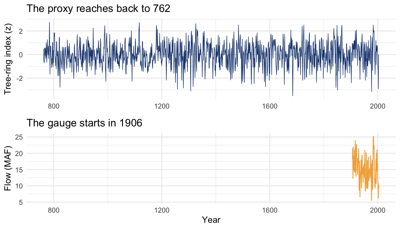

And here are the same data over the instrumental period.

pProxy <- ggplot(instrumental, aes(Year, Proxy)) +
  geom_line(color = bookPal[1], linewidth = 0.3) +
  geom_point(color = bookPal[1], alpha = 0.35) +
  labs(y = "Tree-ring index (z)", x = NULL) +
  theme_minimal()

pFlow <- ggplot(instrumental, aes(Year, ObsMAF)) +
  geom_line(color = bookPal[5], linewidth = 0.3) +
  geom_point(color = bookPal[5], alpha = 0.35) +
  labs(y = "Flow (MAF)", x = "Year") +
  theme_minimal()

pScatter <- ggplot(instrumental, aes(Proxy, ObsMAF)) +
  geom_point(color = bookPal[3], alpha = 0.5) +
  geom_smooth(method = "lm", se = FALSE, color = bookPal[3], linewidth = 0.7) +
  labs(x = "Tree-ring index (z)", y = "Flow (MAF)") +
  theme_minimal()

pSeries <- cowplot::plot_grid(pProxy, pFlow, ncol = 1, align = "v")
cowplot::plot_grid(pSeries, pScatter, ncol = 2, rel_widths = c(1.3, 1))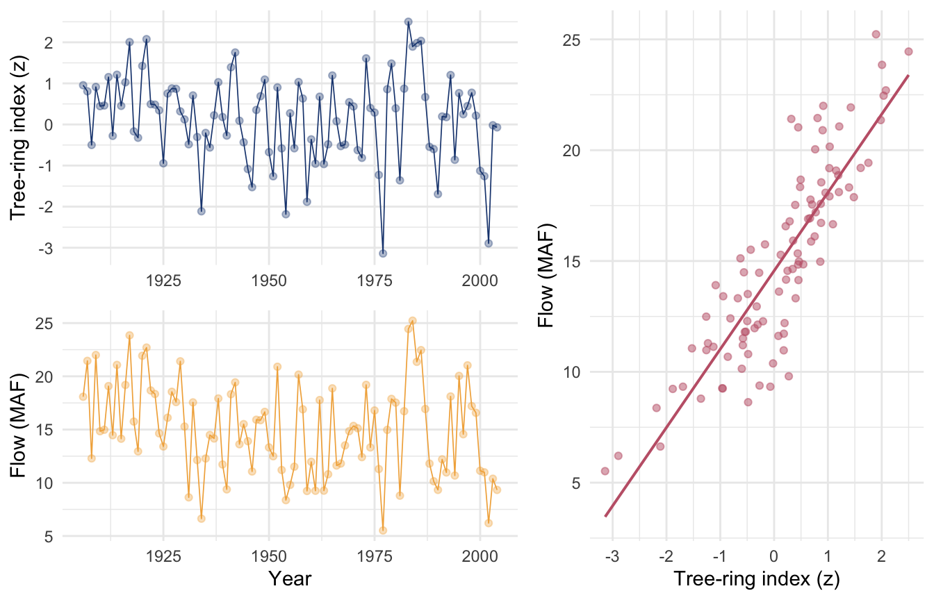

This is a stunning match between tree growth and river flow. And before we go any further let’s look at the autocorrelation in these data over the instrumental record.

pProxyACF <- ggAcf(instrumental$Proxy) +
  labs(title = "Proxy data") +
  theme_minimal()

pFlowACF <- ggAcf(instrumental$ObsMAF) +
  labs(title = "Flow data") +
  theme_minimal()

cowplot::plot_grid(pProxyACF,
  pFlowACF,
  ncol = 2, align = "v")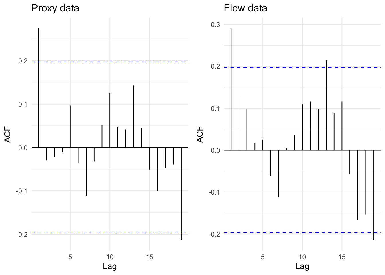

Both show a significant AR(1) process. We’ll have to keep that in mind as we continue to build a model.

So, if the rings track flow over the ninety-nine years where we can compare them, we can run the relationship backward and estimate flow for the twelve centuries where we cannot. The relationship is just a regression, ObsMAF ~ Proxy, the same tool from two chapters ago.

One thing worth being clear about before we fit anything. Writing ObsMAF ~ Proxy puts flow on the left and the tree rings on the right, and a regression like that often reads as effect on cause. Is that the claim, that tree growth causes the river to rise and fall? No. Both are downstream of the same cause, the winter snowpack and basin-wide moisture in a given year. A wide ring and a big flow year are two instruments recording the same weather, not one causing the other. The proxy sits on the right because it is the one thing we have for the centuries before any gauge existed, not because it drives the flow. That makes this a calibration, not a causal model. A strong \(R^2\) here tells you the rings and the river are reading the same climate. It tells you nothing about which one, if either, is in charge.

Calibration and Verification

The tempting move is to fit the regression on all ninety-nine instrumental years and start reconstructing. Do not. A model graded on the same data that trained it will always look better than it is, because it has already seen the answers. The number that matters is how it does on data it has never met. So we split the instrumental record in two. We calibrate the model on one half and verify it on the other, predicting flow for years that took no part in the fit.

calib <- instrumental |> filter(Year <= 1955)
verif <- instrumental |> filter(Year >= 1956)

model <- lm(ObsMAF ~ Proxy, data = calib)
verif <- verif |> mutate(pred = predict(model, verif))

Before we score anything, look at the residuals, the same discipline the regression chapter insisted on. Both the proxy and the flow record carry their own year-to-year memory: a wet year tends to follow a wet year, and a wide ring tends to follow a wide ring, because soil moisture and stored carbohydrates both carry over. So you would be right to worry that the calibration model’s errors carry that same memory, which would mean we have fewer independent years of evidence than the count of ninety-nine suggests.

ggAcf(residuals(model)) +
  labs(title = "ACF of calibration-model residuals") +
  theme_minimal()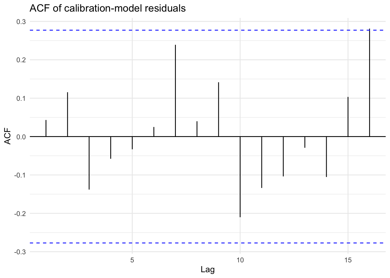

Unlike the raw data, nothing crosses the band. These are the kind of numbers chance alone would produce. This is the ozone resolution from the regression chapter all over again: it is fine for the inputs to a regression to carry memory, what has to come out clean is what is left over once the line is fit. Here the proxy is doing the job temperature did for ozone. Both the rings and the river are responding to the same winter snowpack and spring runoff, so once the proxy is in the model there is no shared climate signal left for the residuals to inherit. A quick GLS fit confirms it.

glsModel <- gls(ObsMAF ~ Proxy, data = calib, correlation = corAR1())
summary(glsModel)

Generalized least squares fit by REML
  Model: ObsMAF ~ Proxy 
  Data: calib 
       AIC      BIC    logLik
  230.9269 238.4117 -111.4634

Correlation Structure: AR(1)
 Formula: ~1 
 Parameter estimate(s):
       Phi 
0.07835457 

Coefficients:
                Value Std.Error  t-value p-value
(Intercept) 14.820231 0.3595354 41.22051       0
Proxy        3.547026 0.3494127 10.15139       0

 Correlation: 
      (Intr)
Proxy -0.234

Standardized residuals:
        Min          Q1         Med          Q3         Max 
-2.61668075 -0.64302713 -0.02314921  0.77335588  2.38431950 

Residual standard error: 2.288857 
Degrees of freedom: 50 total; 48 residual

The estimated AR(1) parameter comes back near zero, and the slope and its standard error barely move from the OLS fit. GLS has nothing to fix here, so we will not drag the rest of the chapter through it. Check, don’t assume, and here the check says OLS already had it right. If you reconstruct something where that check fails, that is exactly when you would reach for gls the way the regression chapter did.

Now we need a way to score the prediction. The natural question is whether the model does better than the dumbest defensible guess you could make, which is to ignore the proxy entirely and predict every year as the average flow. Two statistics from the paleoclimate literature put a number on exactly that, and both are simple enough to write by hand.

The reduction of error, RE, compares the model’s squared errors against what you would get by guessing the calibration period mean for every verification year. The idea is to calibrate a proxy against a short instrumental record, then ask whether it earns its keep on years it never saw. Fritts and colleagues worked the statistic into standard dendroclimatology practice through the 1970s and 1980s, and it has been a fixture of reconstruction papers ever since (Cook and Kairiukstis 1990). The coefficient of efficiency, CE, does the same but against the verification period mean, which is a stiffer test because that mean is the best flat number you could have used for the years being predicted. CE did not grow up in dendrochronology at all: it is the Nash-Sutcliffe efficiency, imported wholesale from hydrology, where it has graded rainfall-runoff models since 1970 (Nash and Sutcliffe 1970). Different fields landed on the same arithmetic because they were asking the same question, how much better is the model than guessing a constant, on data the model never trained on.

skill <- function(obs, pred, calibMean) {
  sse <- sum((obs - pred)^2)
  RE <- 1 - sse / sum((obs - calibMean)^2)   # vs the calibration-period mean
  CE <- 1 - sse / sum((obs - mean(obs))^2)     # vs the verification-period mean
  c(RE = RE, CE = CE)
}

obsSkill <- skill(verif$ObsMAF, verif$pred, calibMean = mean(calib$ObsMAF))
obsSkill

       RE        CE 
0.8050336 0.7887489 

Both come back well above zero. An RE or CE of zero means the model is no better than guessing the mean; anything above zero means it has skill on years it never saw, and one means perfect prediction. Getting a CE comfortably above zero is the result you want, because it is the harder of the two to clear. A model can post a high calibration \(R^2\) and still fail here, and if it did, that would be the model telling you it had memorized the calibration period rather than learned anything that travels. This one travels.

But “above zero” is doing a lot of work in that sentence, so ask the obvious question: is zero actually a high bar? Neither RE nor CE has a textbook sampling distribution the way a correlation or an \(R^2\) does. There is no summary() table with a p-value attached, because the statistic is not built from a model with known degrees of freedom, it is built from comparing two sums of squared errors with no assumed distribution behind either one. For most of the history of these statistics, the field’s working answer was the threshold itself: above zero counts as skill.

That answer is not always safe. Macias-Fauria et al. (2012) showed that an autocorrelated proxy can clear zero by chance more often than the plain threshold assumes, for the same reason chapter eight warned about: persistence lets a relationship look stronger than it is, because the calibration and verification years are not as independent as their count suggests. The fix is the habit this book keeps coming back to. Don’t trust the threshold. Build the null distribution yourself: simulate a proxy with no actual relationship to flow but the same year-to-year persistence as the one we have, run it through the identical calibration and verification, and see how often a meaningless proxy could produce an RE or CE this large.

phiProxy <- acf(instrumental$Proxy, plot = FALSE)$acf[2]
nCal <- nrow(calib)
nVer <- nrow(verif)
nTot <- nCal + nVer

nSim <- 2000
nullRE <- numeric(nSim)
nullCE <- numeric(nSim)
for (i in 1:nSim) {
  fakeProxy <- arima.sim(list(ar = phiProxy), n = nTot)
  m <- lm(calib$ObsMAF ~ fakeProxy[1:nCal])
  pred <- coef(m)[1] + coef(m)[2] * fakeProxy[(nCal + 1):nTot]
  s <- skill(verif$ObsMAF, pred, calibMean = mean(calib$ObsMAF))
  nullRE[i] <- s["RE"]
  nullCE[i] <- s["CE"]
}

c(nullREMax = max(nullRE), nullCEMax = max(nullCE))

nullREMax nullCEMax 
0.1754816 0.1066130 

phiProxy is the lag-1 autocorrelation of the tree-ring index itself, about 0.27, so every simulated proxy carries the same persistence as the one we actually have without carrying any information about flow. Two thousand of them, and none come close. The best a meaningless, equally persistent proxy could manage was an RE of 0.18 and a CE of 0.11, nowhere near the 0.81 and 0.79 this proxy actually earned. So yes, these numbers are good, and now that conclusion comes from a Monte Carlo test. It is also worth noticing why the rule of thumb held up here: this proxy’s persistence is mild. Run the same check on a more autocorrelated proxy and the safe threshold creeps up well past zero, which is exactly the point Macias-Fauria et al. (2012) make. Zero is not a law of nature, just a threshold that needs checking like anything else in this book.

There is nothing special about calibrating on the early half and verifying on the late half, so we should check it the other way too. Swapping the roles is standard practice, and a reconstruction you can trust should pass in both directions.

validate <- function(cal, ver) {
  m <- lm(ObsMAF ~ Proxy, data = cal)
  pred <- predict(m, ver)
  c(calibR2 = summary(m)$r.squared,
    skill(ver$ObsMAF, pred, calibMean = mean(cal$ObsMAF)))
}

bind_rows(
  `calibrate early, verify late` = validate(calib, verif),
  `calibrate late, verify early` = validate(verif, calib),
  .id = "split"
)

# A tibble: 2 × 4
  split                        calibR2    RE    CE
  <chr>                          <dbl> <dbl> <dbl>
1 calibrate early, verify late   0.689 0.805 0.789
2 calibrate late, verify early   0.804 0.701 0.668

Positive RE and positive CE in both directions. This is the same move the forecasting chapter made when it withheld the tail of a series and predicted it, only now we are running it backward in time: holding out years, predicting them from the proxy, and checking. The model earns its trust on data it was not allowed to learn from, which is the only kind of trust worth having. Now, and only now, we reconstruct.

The Reconstruction

With the relationship validated, we refit it on the whole instrumental period to use every year of information we have, and apply it to the full twelve centuries of proxy.

finalModel <- lm(ObsMAF ~ Proxy, data = instrumental)
coef(finalModel)

(Intercept)       Proxy 
  14.557266    3.533699 

coRiverFlow <- coRiverFlow |>
  mutate(recon = predict(finalModel, coRiverFlow),
    reconSmooth = slide_dbl(recon, mean, .before = 12, .after = 12,
      .complete = TRUE))

The fitted relationship is ObsMAF \(= 14.6 + 3.5 \times \text{proxy}\), in millions of acre-feet. Running it across the whole proxy gives an estimate of Colorado River flow for every year since 762. The annual reconstruction is noisy, so we overlay a 25-year centered running mean to bring out the slow swings, the droughts and pluvials that play out over decades.

ggplot(coRiverFlow, aes(Year)) +
  geom_line(aes(y = recon), color = bookPal[1], linewidth = 0.2, alpha = 0.6) +
  geom_line(aes(y = reconSmooth), color = bookPal[5], linewidth = 0.8) +
  geom_hline(yintercept = mean(instrumental$ObsMAF), linetype = "dashed") +
  labs(x = "Year", y = "Reconstructed flow (MAF)",
    title = "Colorado River flow at Lees Ferry, reconstructed from 762",
    subtitle = "Thin line annual, thick line 25-year mean, dashed line the instrumental average") +
  theme_minimal()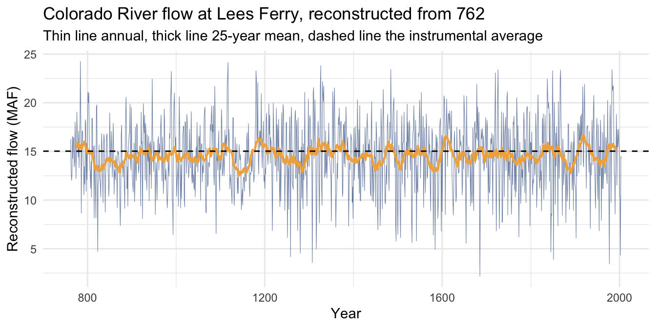

What the Long View Shows

The dashed line is the average flow over the instrumental period, the number everyone who manages the river grew up thinking of as normal. The reconstruction puts it in company, and the company is unflattering. Set the long record against that instrumental baseline.

instMean <- mean(instrumental$ObsMAF)
pctOfNormal <- function(years) {
  round(100 * mean(coRiverFlow$recon[coRiverFlow$Year %in% years]) / instMean)
}

c(fullRecord = pctOfNormal(coRiverFlow$Year),
  compactDecade1912_1921 = pctOfNormal(1912:1921),
  megadrought1130_1154 = pctOfNormal(1130:1154),
  dustBowl1933_1940 = pctOfNormal(1933:1940))

            fullRecord compactDecade1912_1921   megadrought1130_1154 
                    97                    117                     83 
     dustBowl1933_1940 
                    91 

The Colorado River Compact, which still governs how the river is divided among seven states and Mexico, was negotiated in 1922 using flow data from the preceding decade. That decade, 1912 to 1921, ran at 117% of the long-term average. The river was carved up on the basis of one of the wettest stretches in twelve hundred years, and the allocations have been writing checks the river cannot cash ever since. Meanwhile the full twelve-century record averages 97% of the instrumental mean, confirming that the gauged era itself ran a little wet. And the medieval megadrought of the twelfth century, 1130 to 1154, held the river at 83% of normal for a quarter century straight, a sustained drought deeper and longer than anything in the instrumental record, deeper than the Dust Bowl. None of that is visible from ninety-nine years of gauge data. You can only see it because the trees remembered, and you can only believe the trees because the reconstruction earned it in verification.

Stationarity Is Dead

Stationarity Is Dead: Whither Water Management? is the title of an influential policy paper Milly and coauthors had in Science (Milly et al. 2008). Their argument: a warming climate has broken the assumption underneath a century of water engineering, that the statistics measured in the past, the means and variances engineers designed dams and allocations around, are a safe guide to the future. Once a climate is actively warming, that assumption stops holding, and water managers have to learn to plan without it.

So is the Colorado’s reconstructed flow non-stationary, in the sense the paper means? Test it, the way chapter four tested Lake Huron.

adf.test(coRiverFlow$recon)

    Augmented Dickey-Fuller Test

data:  coRiverFlow$recon
Dickey-Fuller = -10.76, Lag order = 10, p-value = 0.01
alternative hypothesis: stationary

kpss.test(coRiverFlow$recon)

    KPSS Test for Level Stationarity

data:  coRiverFlow$recon
KPSS Level = 0.041296, Truncation lag parameter = 7, p-value = 0.1

ADF rejects the unit root, KPSS does not reject stationarity, and a line fit through all twelve hundred years comes back flat, even restricted to the centuries before any gauge existed. By every test in this book, the reconstruction is stationary, sensu stricto: no drift, no unit root, no trend across a thousand years.

None of that shrinks what comes next. Slide a 100-year window across the full twelve centuries and ask how often it would have landed wetter than the one the gauges actually recorded.

roll100 <- slide_dbl(coRiverFlow$recon, mean, .before = 99, .complete = TRUE)
roll100 <- roll100[!is.na(roll100)]
round(100 * mean(roll100 > instMean), 1)

[1] 3.7

Only 3.7% of the windows do. The instrumental record sits near the 96.3th percentile of everything the river has done since 762. A stationary process with this much natural variability can still hand you a deeply misleading 99-year sample, and that is what it did. Water law, reservoir design, and drought planning across the American West were built on that one stretch, mean and variance both, as if it were the river’s settled character. Twelve centuries of tree rings say the stretch was generous, not settled.

Once you can see a thousand years of a river, you can see exactly how unrepresentative the slice anyone has ever gauged turns out to be.

So where does that leave Milly’s actual claim? This record ends in 2004 and has nothing to say about the river since. What it does establish is that a river behaving exactly the way it always had was never the tame, well-behaved system anyone planning around the gauge record assumed. Whether the Colorado has since started to drift the way Milly’s paper warns about is a separate question, and one this record cannot answer, because the proxy stops right where a warming signal would have to show up. Woodhouse et al. (2016) picks up close to where this reconstruction leaves off and finds rising temperature already amplifying drought beyond what precipitation alone predicts, which is the kind of evidence that could eventually tip a river from stationary to not. Maybe stationarity was not dead in 2004, when this record ends. Maybe it is dying now.

And notice what licenses any of this: the verification, not the tree rings on their own and not a confident-looking line through a scatterplot. The reason we can hold a record that sits at the 96th percentile of 100-year draws up against twelve centuries, or set the medieval megadrought next to the Dust Bowl, and take any of it seriously, is that the model behind it cleared an out-of-sample test, twice. Out-of-sample skill is the line between using the past to bound what is possible and merely fitting a curve and trusting your story.

Wrapping Up

The worked example was a streamflow reconstruction, but the chapter was about a habit. Before you trust a model to speak about data it has not seen, whether that is the deep past or next year’s peak demand, you withhold, you predict, and you score the prediction against the plain baseline of guessing the mean. RE and CE are two ways to keep that score, and a model that clears them on held-out data has earned a kind of trust that calibration statistics alone can never grant. The forecasting chapter ran this validation forward into the future; here we ran it backward into the past, and it is the same discipline pointed in two directions. It is also the discipline that turns “the software fit a model” into “I have a result I can stand behind,” which is the whole project of this book.

Exercises

Move the wall

We split the instrumental record at 1955. Redo the validation with the split at 1930 and again at 1980, so that the calibration and verification periods are lopsided rather than even. Do RE and CE stay positive? Then try a harder test: calibrate on the middle of the record and verify on both ends at once. What does it tell you about a reconstruction if its skill depends a lot on where you put the wall, and what would you want to see before trusting it back to the year 762?

Find the pluvials

The chapter dwelt on droughts, but the reconstruction holds wet anomalies too. Using the 25-year running mean, find the wettest quarter-century in the whole record and compare it to the 1912 to 1921 decade that anchored the Compact. Was the decade the river was divided on merely wet, or close to the wettest the river has run in twelve hundred years? Write a sentence you would put in front of a water manager, with the number in it.

Further Reading

• Meko et al. (2007) is the reconstruction this chapter is built on, and it works through the medieval megadrought in the upper basin in detail.
• Woodhouse et al. (2006) lays out the streamflow reconstruction methods for the Colorado in full, including the calibration and verification practice we used here.
• Cook and Kairiukstis (1990) is the standard reference for RE and the rest of the dendroclimatology calibration-verification toolkit.
• Nash and Sutcliffe (1970) is where CE comes from, under its original name, decades before tree-ring scientists borrowed it.
• Macias-Fauria et al. (2012) makes the case in detail that RE and CE need a Monte Carlo significance test, not a zero threshold, once a proxy carries meaningful persistence.